Finite-n Estimate of Dedekind Numbers by Layer-Ratio Monte Carlo
Pith reviewed 2026-06-27 15:49 UTC · model grok-4.3
The pith
Layer-ratio Monte Carlo sampling produces the estimate M(10) = (8.9360 ± 0.0010) × 10^78.
A machine-rendered reading of the paper's core claim, the machinery that carries it, and where it could break.
Core claim
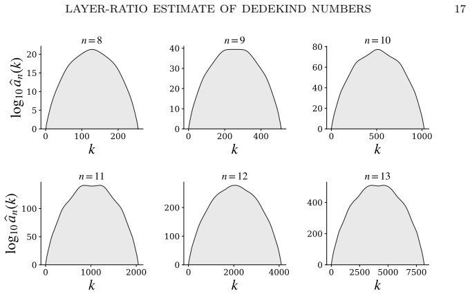
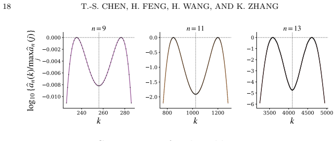
The central claim is that each layer ratio is exactly recoverable from the local averages of addable and removable elements via an adjacent-layer double count, and that reversible fixed-layer Markov chains can estimate those averages with sufficient fidelity to reconstruct the Dedekind numbers. Backtests on M(8) and M(9) establish a cross-n scaling law that forecasts Monte Carlo variability, yielding the production-budget estimate ĤM(10) = (8.9360 ± 0.0010) × 10^78. The same high-precision n=9 reconstruction exhibits a shallow two-shoulder feature around the central rank, contrary to the prior empirical description of unimodality; analogous patterns appear in center-window estimates for n=11
What carries the argument
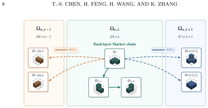
Reversible fixed-layer Markov chains that estimate local averages of addable and removable elements for layer-ratio reconstruction.
If this is right
- The protocol yields the stated numerical estimate for M(10) together with its budget-based uncertainty.
- The Whitney numbers of the ideal lattice at n=9 display a shallow two-shoulder feature around the central rank.
- Center-window estimates at n=11 and n=13 exhibit a larger-contrast version of the same non-unimodal pattern.
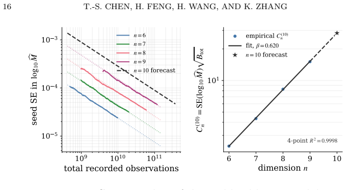
- The cross-n scaling law derived from backtests at n=8 and n=9 supplies the uncertainty scale used at n=10.
- The method supplies the first quantitative probe of the full Whitney-number sequence of the ideal lattice at these sizes.
Where Pith is reading between the lines
- If the scaling law continues to hold, the same protocol could be run at n=11 with a proportionally larger budget to obtain a comparable-precision estimate.
- The reported departure from unimodality invites a re-examination of how the ranks of monotone Boolean functions are distributed for n greater than 9.
- The layer-ratio approach may transfer to other poset-enumeration tasks where adjacent-layer double counting is feasible.
Load-bearing premise
The reversible fixed-layer Markov chains converge sufficiently to produce unbiased estimates of the local averages, and the cross-n scaling law fitted from M(8) and M(9) correctly forecasts variability at n=10.
What would settle it
An independent exact computation or substantially higher-precision simulation of M(10) whose value lies outside the interval (8.9360 ± 0.0010) × 10^78.
Figures
read the original abstract
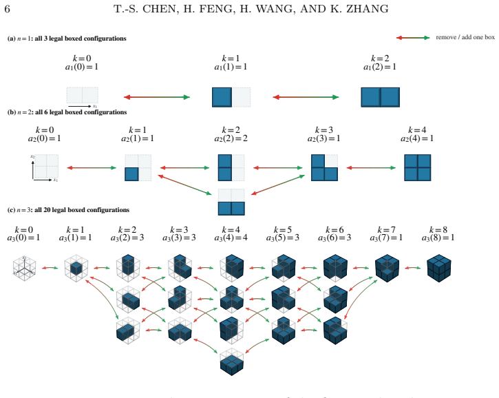
Dedekind's problem counts monotone Boolean functions, equivalently downsets of a Boolean lattice. We recast this enumeration as a finite layer-ratio reconstruction problem for the Whitney numbers of the ranked ideal lattice. An exact adjacent-layer double count expresses each layer ratio through local averages of the number of addable elements and the number of removable elements. Reversible fixed-layer Markov chains estimate these averages and hence estimate the Dedekind number M(n). Backtests at M(8) and M(9) calibrate seed-level variability under the fixed protocol and measure the observed Monte Carlo budget scaling. The resulting estimate probes the Whitney-number sequence of the ideal lattice. Although these rows have previously been described empirically as unimodal, the high-precision n=9 estimate has a shallow two-shoulder feature around the central rank, contrary to that empirical description; n=11 and n=13 center-window estimates show a larger-contrast analogous pattern. The protocol estimate for M(10) is \[ \widehat M(10)=(8.9360\pm0.0010)\times 10^{78}, \] where the displayed uncertainty is the budget-based forecast scale from the cross-n scaling law under the production budget.
Editorial analysis
A structured set of objections, weighed in public.
Referee Report
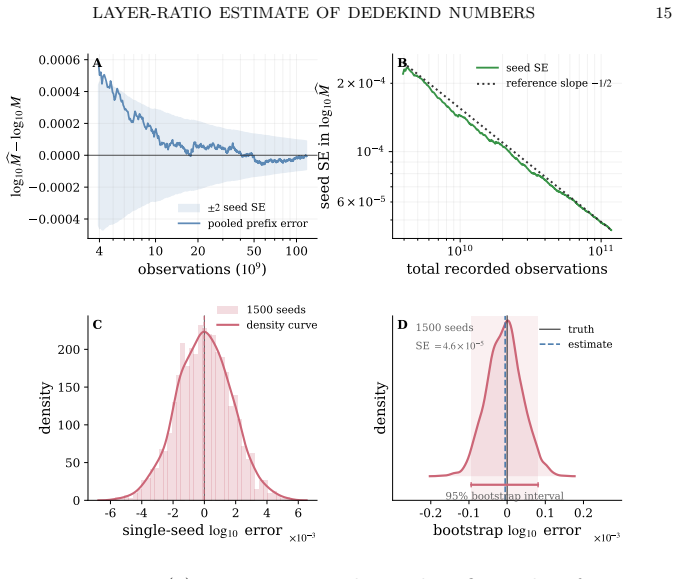
Summary. The paper recasts Dedekind number enumeration M(n) as a finite layer-ratio reconstruction problem on the Whitney numbers of the ranked ideal lattice. It derives an exact adjacent-layer double-count relation expressing each ratio via local averages of addable and removable elements, estimates these averages via reversible fixed-layer Markov chains, backtests the protocol on known M(8) and M(9) to calibrate seed-level variability and a cross-n Monte Carlo budget scaling law, and reports the estimate ĤM(10)=(8.9360±0.0010)×10^78 whose uncertainty is the budget-based forecast from that scaling law. It also notes a shallow two-shoulder feature in the n=9 Whitney numbers contrary to prior unimodality descriptions.
Significance. If the Markov-chain estimates are unbiased and the cross-n scaling law extrapolates reliably, the work supplies a new high-precision value for the previously unknown M(10) together with structural observations on the ideal-lattice Whitney numbers at n=9,11,13. The exact double-count identity provides a clean theoretical foundation, and the backtests on M(8),M(9) constitute a concrete reproducibility check.
major comments (2)
- [Abstract] Abstract: the displayed uncertainty ±0.0010 is obtained solely from a budget-based forecast scale of the cross-n scaling law fitted to the M(8) and M(9) backtests; no independent diagnostic (multiple independent n=10 runs, direct observed-vs-predicted variance comparison, or effective-sample-size analysis) is supplied to confirm that the scaling continues to hold at n=10, rendering the reported precision dependent on an untested extrapolation.
- [The section describing the reversible fixed-layer Markov chains] The section describing the reversible fixed-layer Markov chains: the protocol assumes these chains converge sufficiently to produce unbiased estimates of the local averages of addable and removable elements, yet no mixing-time bounds, convergence diagnostics, or effective-sample-size calculations are reported, which is load-bearing for the correctness of every layer-ratio estimate feeding into ĤM(10).
Simulated Author's Rebuttal
We thank the referee for the careful reading and constructive comments. We respond point-by-point to the major comments below.
read point-by-point responses
-
Referee: [Abstract] Abstract: the displayed uncertainty ±0.0010 is obtained solely from a budget-based forecast scale of the cross-n scaling law fitted to the M(8) and M(9) backtests; no independent diagnostic (multiple independent n=10 runs, direct observed-vs-predicted variance comparison, or effective-sample-size analysis) is supplied to confirm that the scaling continues to hold at n=10, rendering the reported precision dependent on an untested extrapolation.
Authors: We agree that the reported uncertainty for ĤM(10) is a forecast obtained by extrapolating the scaling law fitted to the M(8) and M(9) backtests; no separate n=10 variance diagnostics were computed. The single production run at n=10 was sized according to that law, and the backtests supply the only empirical calibration available under the fixed protocol. We will revise the abstract and methods to state explicitly that the uncertainty is extrapolated rather than directly measured at n=10. revision: yes
-
Referee: [The section describing the reversible fixed-layer Markov chains] The section describing the reversible fixed-layer Markov chains: the protocol assumes these chains converge sufficiently to produce unbiased estimates of the local averages of addable and removable elements, yet no mixing-time bounds, convergence diagnostics, or effective-sample-size calculations are reported, which is load-bearing for the correctness of every layer-ratio estimate feeding into ĤM(10).
Authors: The protocol's practical reliability is evidenced by the backtests, which recover the exact known values of M(8) and M(9) within the stated uncertainties. We acknowledge that the manuscript contains no mixing-time bounds or ESS calculations. In revision we will add autocorrelation times and effective-sample-size estimates computed from the n=9 and n=10 chain trajectories to document convergence under the production budget. revision: yes
Circularity Check
M(10) uncertainty obtained by applying scaling law fitted to n=8,9 backtest variability
specific steps
-
fitted input called prediction
[Abstract]
"the displayed uncertainty is the budget-based forecast scale from the cross-n scaling law under the production budget."
Backtests at M(8) and M(9) are used to calibrate seed-level variability and measure the observed Monte Carlo budget scaling; the scaling law fitted to those data is then applied to forecast the uncertainty attached to the n=10 estimate, so the reported error bar is produced by the calibration fit rather than measured independently at n=10.
full rationale
The central M(10) point estimate is produced by applying the layer-ratio Markov chain protocol directly at n=10. The attached uncertainty, however, is generated by first fitting a cross-n scaling law to the observed Monte Carlo variability measured during backtests at n=8 and n=9, then using that fit to forecast the error scale at the production budget for n=10. This matches the fitted-input-called-prediction pattern for the uncertainty component while leaving the numerical estimate itself independent of the fit. No self-definitional reductions, load-bearing self-citations, or other circular steps appear in the provided derivation chain.
Axiom & Free-Parameter Ledger
free parameters (1)
- cross-n scaling law parameters
axioms (1)
- domain assumption Each layer ratio equals the ratio of local averages of addable and removable elements via an exact adjacent-layer double count.
Reference graph
Works this paper leans on
- [1]
-
[2]
Estimating the size of a set using cascading exclusion
URL:https://arxiv.org/abs/ 2508.05901,arXiv:2508.05901. [Chu40] Randolph Church. Numerical analysis of certain free distributive struc- tures.Duke Mathematical Journal, 6(3):732–734,
work page internal anchor Pith review Pith/arXiv arXiv
-
[3]
On the number of antichains of sets in a finite universe
URL:https://arxiv.org/abs/ 1407.4288,arXiv:1407.4288. LAYER-RATIO ESTIMATE OF DEDEKIND NUMBERS 21 [DCVH26] Patrick De Causmaecker and Lennart Van Hirtum. Solving systems of equations on antichains for the computation of the ninth Dedekind number. Journal of Combinatorial Optimization, 51(1),
work page internal anchor Pith review Pith/arXiv arXiv
-
[4]
20904,doi:10.1007/s10878-025-01361-9
Article 5.arXiv:2405. 20904,doi:10.1007/s10878-025-01361-9. [Ded97] Richard Dedekind. Über zerlegungen von zahlen durch ihre grössten gemein- samen theiler. InFest-Schrift der Herzoglichen Technischen Hochschule Carolo-Wilhelmina, pages 1–40. Vieweg+Teubner Verlag,
-
[5]
URL: https://arxiv.org/abs/cond-mat/9610041,arXiv:cond-mat/9610041. [Eng97] Konrad Engel.Sperner Theory. Cambridge University Press, Cambridge, 1997.doi:10.1017/CBO9780511574719. [ET93] Bradley Efron and Robert J. Tibshirani.An Introduction to the Bootstrap. Chapman & Hall/CRC, New York, 1993.doi:10.1201/9780429246593. [FMSS01] Robert Fidytek, Andrzej W. ...
work page internal anchor Pith review Pith/arXiv arXiv doi:10.1017/cbo9780511574719 1997
-
[6]
[FRRT26] Victor Falgas-Ravry, Eero Räty, and István Tomon
doi:10.1016/S0020-0190(00) 00230-1. [FRRT26] Victor Falgas-Ravry, Eero Räty, and István Tomon. Dedekind’s problem in the hypergrid.Advances in Mathematics, 488:110796, 2026.arXiv:2310. 12946,doi:10.1016/j.aim.2026.110796. [GK76] Curtis Greene and Daniel J. Kleitman. Strong versions of Sperner’s theorem. Journal of Combinatorial Theory, Series A, 20(1):80–...
-
[7]
Counting maximal antichains and independent sets
arXiv:1202.4427, doi:10.1007/ s11083-012-9253-5. [Inc26] The OEIS Foundation Inc. A269699: Irregular triangle read by rows: number of k-element proper ideals of then-dimensional Boolean lattice. The On- Line Encyclopedia of Integer Sequences,
work page internal anchor Pith review Pith/arXiv arXiv
-
[8]
Entry A269699. URL:https: //oeis.org/A269699. [Jäk23] Christian Jäkel. A computation of the ninth Dedekind number.Journal of Computational Algebra, 6–7:100006, 2023.arXiv:2304.00895, doi:10. 1016/j.jaca.2023.100006. [JMP24] Matthew Jenssen, Alexandru Malekshahian, and Jinyoung Park. On Dedekind’s problem, a sparse version of Sperner’s theorem, and anticha...
-
[9]
[JPS26] Matthew Jenssen, Jinyoung Park, and Michail Sarantis
URL:https://arxiv.org/abs/ 2411.03400,arXiv:2411.03400. [JPS26] Matthew Jenssen, Jinyoung Park, and Michail Sarantis. On the number of antichains in{0,1,2}n,
-
[10]
URL:https://arxiv.org/abs/2601.07650, arXiv:2601.07650. [Kah02] Jeff Kahn. Entropy, independent sets and antichains: a new approach to Dedekind’s problem.Proceedings of the American Mathematical Society, 130(2):371–378, 2002.doi:10.1090/S0002-9939-01-06058-0. [Kle69] Daniel J. Kleitman. On Dedekind’s problem: the number of monotone Boolean functions.Proce...
-
[11]
[Kor77] A
doi:10.1090/ s0002-9947-1975-0382107-0. [Kor77] A. D. Korshunov. Solution of Dedekind’s problem on the number of mono- tonic Boolean functions.Doklady Akademii Nauk SSSR, 233(4):543–546,
1975
-
[12]
URL:https://www.mathnet.ru/eng/dan40395
English translation: Soviet Mathematics Doklady 18 (1977), 442–445. URL:https://www.mathnet.ru/eng/dan40395. [Kor03] A. D. Korshunov. Monotone Boolean functions.Russian Mathematical Surveys, 58(5):929–1001, 2003.doi:10.1070/rm2003v058n05abeh000667. [KS02] A. D. Korshunov and I. Shmulevich. On the distribution of the number of monotone Boolean functions re...
-
[13]
doi:10.1090/mbk/058. [Mac99] P. A. MacMahon. Memoir on the theory of the partitions of numbers. Part II.Proceedings of the Royal Society of London, 64(402–411):224–227,
-
[14]
doi:10.1098/rspl.1898.0095. [Mac12] P. A. MacMahon. Ix. memoir on the theory of the partitions of numbers. Part VI. partitions in two-dimensional space, to which is added an adumbration of the theory of the partitions in three-dimensional space.Philosophical Transactions of the Royal Society of London. Series A, 211(471–483):345– 373, 1912.doi:10.1098/rst...
-
[15]
URL:https://escholarship.org/uc/item/8wh6f7rc. [MRR+53] Nicholas Metropolis, Arianna W. Rosenbluth, Marshall N. Rosenbluth, Augusta H. Teller, and Edward Teller. Equation of state calculations by fast computing machines.Journal of Chemical Physics, 21(6):1087–1092, 1953.doi:10.1063/1.1699114. [Paw22] Bartłomiej Pawelski. On the number of inequivalent mono...
-
[16]
URL: https://cs.uwaterloo.ca/journals/JIS/VOL25/Pawelski/ pawelski7.html
Article 22.7.7. URL: https://cs.uwaterloo.ca/journals/JIS/VOL25/Pawelski/ pawelski7.html. [Paw24] Bartłomiej Pawelski. On the number of inequivalent monotone Boolean func- tions of 9 variables.IEEE Transactions on Information Theory, 70(7):5358– 5364, 2024.doi:10.1109/TIT.2024.3379594. [PS23] Bartłomiej Pawelski and Andrzej Szepietowski. Divisibility prop...
-
[17]
URL: https://cs.uwaterloo.ca/journals/JIS/VOL28/Pawelski/ pawelski22.html
Article 25.6.5. URL: https://cs.uwaterloo.ca/journals/JIS/VOL28/Pawelski/ pawelski22.html. [PSS80] Robert A. Proctor, Michael E. Saks, and Dean G. Sturtevant. Product partial orders with the Sperner property.Discrete Mathematics, 30(2):173– 180, 1980.doi:10.1016/0012-365X(80)90118-1. LAYER-RATIO ESTIMATE OF DEDEKIND NUMBERS 23 [PST25] Jinyoung Park, Micha...
-
[18]
URL: https://escholarship.org/uc/item/1cp4b92v, arXiv: 2305.16520,doi:10.5070/c65165018. [Sta86] Richard P. Stanley.Enumerative Combinatorics, volume 1 ofThe Wadsworth & Brooks/Cole Mathematics Series. Wadsworth & Brooks/Cole, Monterey, CA, 1986.doi:10.1007/978-1-4615-9763-6. [SY14] Tamon Stephen and Timothy Yusun. Counting inequivalent monotone Boolean f...
-
[19]
arXiv:2304.03039,doi:10.1145/3674147. [War46] Morgan Ward. Note on the order of the free distributive lattice.Bulletin of the American Mathematical Society, 52(5):423,
-
[20]
Abstract 135.doi: 10.1090/s0002-9904-1946-08566-3. [Wie91] Doug Wiedemann. A computation of the eighth Dedekind number.Order, 8(1):5–6, 1991.doi:10.1007/BF00385808. [XFZ+26] Shang Xiang, Hao Feng, Keyou Zhuo, Tian-Shun Chen, and Kilar Zhang. Charge functions for odd dimensional partitions.Journal of High Energy Physics, 2026(5):141,
-
[21]
Charge functions for odd dimensional partitions
URL: https://arxiv.org/abs/2512.07758, arXiv:2512.07758,doi:10.1007/JHEP05(2026)141. [Yam54] Koichi Yamamoto. Logarithmic order of free distributive lattice.Journal of the Mathematical Society of Japan, 6(3–4):343–353, 1954.doi:10.2969/ jmsj/00630343. AppendixA.Protocol and Numerical V alidation Details This appendix records theM(10)production protocol an...
work page internal anchor Pith review Pith/arXiv arXiv doi:10.1007/jhep05(2026)141 2026
-
[22]
Each chain records75post-burn-in states, using burn-in2500and thinning40
(2) Fixed-layer chain layout.For each sampled layer, the protocol runs 4×2048 = 8192fixed-layer chains. Each chain records75post-burn-in states, using burn-in2500and thinning40. Each chain is initialized by starting from the empty downset and adding uniformly chosen addable vertices until the target layerkis reached. (3) Fixed-layer transition.Within a sa...
2048
-
[23]
Accumulate log Whitney numbers from the endpoint: x0,s= 0, x k,s= k−1∑ j=0 ˆyj,s (1≤k≤512)
Form the adjacent log-ratios on the sampled side: ˆyk,s= log ˆAk,s−logˆRk+1,s,0≤k<512. Accumulate log Whitney numbers from the endpoint: x0,s= 0, x k,s= k−1∑ j=0 ˆyj,s (1≤k≤512). Complete the full row by exact rank duality: ˆxk,s= { xk,s,0≤k≤512, x1024−k,s,512<k≤1024. The seed-level reconstructed Whitney numbers are ˆa10,s(k) = exp(ˆxk,s). The seed-level ...
2048
-
[24]
Here(b,t)is the burn-in/thinning pair
Entries compare meanlog10 errors using the same 40 seeds in each setting. Here(b,t)is the burn-in/thinning pair. Comparison Mean diff. SEzMax abs. diff. (5000,80)−(2500,40)−1.7455×10⁻³ 1.3538×10⁻³ −1.29 1.7668×10⁻² (10000,120)−(2500,40) 4.6248×10⁻⁴ 1.0337×10⁻³ 0.45 1.9154×10⁻² (10000,120)−(5000,80) 2.2080×10⁻³ 1.3151×10⁻³ 1.68 1.9773×10⁻² nFormula Exact A...
2080
discussion (0)
Sign in with ORCID, Apple, or X to comment. Anyone can read and Pith papers without signing in.