Recognition: unknown
Beyond the Bellman Fixed Point: Geometry and Fast Policy Identification in Value Iteration
Pith reviewed 2026-05-10 05:49 UTC · model grok-4.3
The pith
Q-value iteration enters a tube around the optimal Q-function in finite time, making the greedy policy optimal before full convergence.
A machine-rendered reading of the paper's core claim, the machinery that carries it, and where it could break.
Core claim
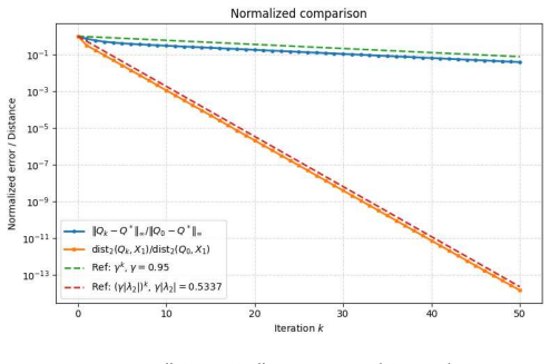
Q-VI reaches the optimal action class in finite time by entering an invariant tube around X1 = Q* + span(1), which is contained in the practically optimal solution set. For every ε > 0 the distance to X1 satisfies an exponential bound with rate (ρ-bar + ε)^k, where ρ-bar is the joint spectral radius of the projected switching family restricted to directions transverse to X1. When ρ-bar < γ this transverse convergence is faster than the classical contraction rate. The analysis separates fast policy identification from the subsequent convergence to Q*, which may still be governed by the all-ones mode.
What carries the argument
The invariant tube around the affine subspace X1 = Q* + span(1) that is contained in the practically optimal solution set, together with the joint spectral radius of the projected switching family of greedy-policy operators restricted to the subspace transverse to the constants.
If this is right
- The greedy policy extracted from the current Q-estimate becomes optimal as soon as the iterate enters the tube, even while the distance to Q* is still large.
- The rate at which the optimal action class is reached is governed by the transverse joint spectral radius and can be strictly smaller than the discount factor γ.
- Spectral and graph-theoretic conditions on the MDP determine whether the strict inequality ρ-bar < γ holds.
- After policy identification, further convergence inside the tube can still be limited by the all-ones eigenvector at the classical rate γ.
Where Pith is reading between the lines
- Early-stopping rules could monitor distance to the tube rather than the full Bellman residual.
- The same transverse-spectral analysis may extend to asynchronous or approximate value iteration variants.
- MDP instances satisfying the graph-theoretic conditions for ρ-bar < γ could be preferentially chosen or constructed to accelerate policy learning.
- The separation of timescales suggests that policy-gradient or actor-critic methods might also benefit from explicit tube geometry around optimal action sets.
Load-bearing premise
Discounted Q-value iteration can be modeled as a switching system whose modes are the greedy policies, and an invariant tube around X1 exists inside the set of Q-functions that induce optimal policies.
What would settle it
A finite MDP in which the sequence of Q-iterates never enters any bounded neighborhood of Q* + span(1) yet the greedy policies extracted along the way remain suboptimal for infinitely many steps.
Figures


read the original abstract
Q-value iteration (Q-VI) is usually analyzed through the \(\gamma\)-contraction of the Bellman operator. This argument proves convergence to \(Q^*\), but it gives only a coarse account of when the induced greedy policy becomes optimal. We study discounted Q-VI as a switching system and focus on the practically optimal solution set (POSS), the set of \(Q\)-functions whose tie-broken greedy policies are optimal. The main result shows that Q-VI reaches the optimal action class in finite time by entering an invariant tube around \(\mathcal X_1=Q^*+\operatorname{span}(\mathbf 1)\), which is contained in the POSS. For every \(\varepsilon>0\), the distance to \(\mathcal X_1\) satisfies an exponential bound with rate \((\bar\rho+\varepsilon)^k\), where \(\bar\rho\) is the joint spectral radius of the projected switching family restricted to directions transverse to \(\mathcal X_1\). When \(\bar\rho<\gamma\), this transverse convergence is faster than the classical contraction rate. The analysis separates fast policy identification from the subsequent convergence to \(Q^*\), which may still be governed by the all-ones mode. We also give spectral and graph-theoretic conditions under which the strict inequality \(\bar\rho<\gamma\) holds or fails.
Editorial analysis
A structured set of objections, weighed in public.
Referee Report
Summary. The paper models discounted Q-value iteration as a switching system whose modes are the greedy policies with respect to the current Q-function. It defines the practically optimal solution set (POSS) as the set of Q-functions whose tie-broken greedy policies are optimal, and shows that Q-VI enters an invariant tube of small transverse radius around the affine line X1 = Q* + span(1) in finite time; this tube lies inside the POSS. Inside the tube the active modes are optimal policies, each of which leaves X1 invariant, and the transverse dynamics on the quotient space are governed by a switching family whose joint spectral radius ρ-bar satisfies ρ-bar ≤ γ. Consequently the transverse distance to X1 contracts at rate (ρ-bar + ε)^k for any ε > 0, which is strictly faster than the classical γ-rate whenever ρ-bar < γ. Spectral and graph-theoretic conditions are supplied under which the strict inequality holds.
Significance. If the central claims hold, the work supplies a geometrically precise account of the finite-time policy-identification phase of Q-VI that is separated from the subsequent convergence to Q*. The decomposition into longitudinal and transverse components, the explicit construction of an invariant tube inside the POSS, and the use of the joint spectral radius to obtain a potentially tighter transverse rate constitute a genuine advance over the standard contraction argument. The provision of verifiable conditions for ρ-bar < γ is a concrete strength that makes the result falsifiable and potentially useful for algorithm analysis.
major comments (2)
- [§3.2] §3.2 (Tube invariance): The proof that any sufficiently small transverse perturbation keeps the argmax set inside the optimal actions relies on a uniform positive gap between optimal and suboptimal action values at Q*. The manuscript should state explicitly that this gap is positive and uniform because the state and action spaces are finite; without that sentence the invariance argument is incomplete for the general case.
- [§4.1] §4.1 (Definition of the projected switching family): The joint spectral radius ρ-bar is defined on the quotient space transverse to X1. The paper must verify that each optimal policy induces a well-defined linear map on this quotient (i.e., that T_π maps X1 to itself) and that the family is finite; both facts are used to bound ρ-bar ≤ γ and should be recorded as a short lemma.
minor comments (3)
- [§2] The notation X1, POSS, and the transverse projection operator are introduced without a small illustrative example (e.g., a two-state chain); adding one would make the geometric construction easier to follow.
- [Theorem 1] Theorem 1 states the exponential bound with rate (ρ-bar + ε)^k; the proof should cite the precise definition of joint spectral radius used (e.g., the one based on the spectral radius of the semigroup or the max-norm growth rate) so that readers can verify the ε-approximation step.
- [§5] The graph-theoretic conditions in §5 are stated for the case of a single optimal policy; the manuscript should note whether the same spectral test extends immediately to multiple optimal policies or requires an additional union-graph construction.
Simulated Author's Rebuttal
We thank the referee for the careful reading and constructive comments. The suggested clarifications strengthen the presentation, and we will incorporate them in the revised version.
read point-by-point responses
-
Referee: [§3.2] §3.2 (Tube invariance): The proof that any sufficiently small transverse perturbation keeps the argmax set inside the optimal actions relies on a uniform positive gap between optimal and suboptimal action values at Q*. The manuscript should state explicitly that this gap is positive and uniform because the state and action spaces are finite; without that sentence the invariance argument is incomplete for the general case.
Authors: We agree that the argument for tube invariance relies on a uniform positive gap, which holds because the finite state-action space implies a positive minimum gap between optimal and suboptimal Q*-values. We will add an explicit sentence in §3.2 stating this fact to make the invariance proof self-contained. revision: yes
-
Referee: [§4.1] §4.1 (Definition of the projected switching family): The joint spectral radius ρ-bar is defined on the quotient space transverse to X1. The paper must verify that each optimal policy induces a well-defined linear map on this quotient (i.e., that T_π maps X1 to itself) and that the family is finite; both facts are used to bound ρ-bar ≤ γ and should be recorded as a short lemma.
Authors: We will add a short lemma in §4.1 that records these two facts: (i) every optimal policy π* satisfies T_π*(Q* + c·1) = Q* + γc·1, so the induced map is well-defined on the quotient transverse to X1, and (ii) the switching family is finite because there are only finitely many deterministic policies. This lemma directly supports the subsequent bound ρ-bar ≤ γ. revision: yes
Circularity Check
No significant circularity; derivation is self-contained
full rationale
The paper analyzes Q-VI via switching systems and the joint spectral radius of the transverse projected family, a standard external concept from control theory. The invariant tube inside the POSS follows from the uniform action gap at Q* (finite actions) plus classical γ-contraction; once inside, optimal modes map the line X1 to itself and the transverse dynamics are bounded by the JSR by definition. No parameter is fitted to the target rate, no self-citation supplies a load-bearing uniqueness theorem, and no step renames or re-derives its own input. The claimed faster transverse rate when ρ-bar < γ is a direct consequence of the JSR definition applied to the quotient space, not a construction internal to the paper.
Axiom & Free-Parameter Ledger
axioms (2)
- domain assumption Discounted Q-value iteration can be represented as a finite switching system whose modes correspond to greedy policies
- ad hoc to paper There exists an invariant tube around X1 = Q* + span(1) that is contained in the practically optimal solution set
invented entities (3)
-
Practically Optimal Solution Set (POSS)
no independent evidence
-
Invariant tube around X1
no independent evidence
-
Joint spectral radius of the projected switching family (transverse to X1)
no independent evidence
Forward citations
Cited by 1 Pith paper
-
Switching-Geometry Analysis of Deflated Q-Value Iteration
Deflated Q-VI is algebraically equivalent to recentering standard Q-VI, yet its error dynamics are governed by the joint spectral radius of a projected switching system that can be strictly smaller than the discount factor γ.
Reference graph
Works this paper leans on
-
[1]
Dynamic programming,
R. Bellman, “Dynamic programming,” science, vol. 153, no. 3731, pp. 34–37, 1966. 10 Figure 4: Orthogonal projections of 12 full Q-VI trajectories onto the tilted plane, where the init ial conditions are chosen uniformly on a circle of radius 2 in the plane. The dashed line is the slice of X1, the shaded strip is the slice of Tδ, and the dotted curve is th...
1966
-
[2]
D. P . Bertsekas and J. N. Tsitsiklis, Neuro-dynamic programming. Athena Scientific Belmont, MA, 1996
1996
-
[3]
Dynamic programming and optimal contr ol 4th edition, volume ii,
D. P . Bertsekas, “Dynamic programming and optimal contr ol 4th edition, volume ii,” Athena Scientific , 2015
2015
-
[4]
M. L. Puterman, Markov decision processes: Discrete stochastic dynamic programming. John Wiley & Sons, 2014
2014
-
[5]
R. S. Sutton and A. G. Barto, Reinforcement learning: An introduction . MIT Press, 1998
1998
-
[6]
Liberzon, Switching in systems and control
D. Liberzon, Switching in systems and control . Springer Science & Business Media, 2003
2003
-
[7]
Stability and stabilizabili ty of switched linear systems: a survey of recent results,
H. Lin and P . J. Antsaklis, “Stability and stabilizabili ty of switched linear systems: a survey of recent results,” IEEE Transactions on Automatic control, vol. 54, no. 2, pp. 308–322, 2009
2009
-
[8]
Resilient stabilization of sw itched linear control systems against adversarial switching,
J. Hu, J. Shen, and D. Lee, “Resilient stabilization of sw itched linear control systems against adversarial switching,” IEEE Transactions on Automatic Control, vol. 62, no. 8, pp. 3820–3834, 2017
2017
-
[9]
Nonlinear systems,
H. K. Khalil, “Nonlinear systems,” Upper Saddle River , 2002
2002
-
[10]
The Lyapunov expone nt and joint spectral radius of pairs of matrices are hard—when not impossible—to compute and to a pproximate,
J. N. Tsitsiklis and V . D. Blondel, “The Lyapunov expone nt and joint spectral radius of pairs of matrices are hard—when not impossible—to compute and to a pproximate,” Mathematics of Control, Signals and Systems , vol. 10, no. 1, pp. 31–40, 1997
1997
-
[11]
A note on the joint spectral ra dius,
G.-C. Rota and G. Strang, “A note on the joint spectral ra dius,” Indag. Math, vol. 22, no. 4, pp. 379–381, 1960
1960
-
[12]
Computationally efficie nt approximations of the joint spectral radius,
V . D. Blondel and Y . Nesterov, “Computationally efficie nt approximations of the joint spectral radius,” SIAM Journal on Matrix Analysis and Applications , vol. 27, no. 1, pp. 256–272, 2005
2005
-
[13]
Central limit theorem for nonstation ary Markov chains. I,
R. L. Dobrushin, “Central limit theorem for nonstation ary Markov chains. I,” Theory of Prob- ability and Its Applications , vol. 1, no. 1, pp. 65–80, 1956
1956
-
[14]
Weak ergodicity in non-ho mogeneous Markov chains,
J. Hajnal and M. S. Bartlett, “Weak ergodicity in non-ho mogeneous Markov chains,” in Math- ematical Proceedings of the Cambridge Philosophical Socie ty, vol. 54, no. 2, 1958, pp. 233– 246
1958
-
[15]
Products of indecomposable, aperiodic , stochastic matrices,
J. Wolfowitz, “Products of indecomposable, aperiodic , stochastic matrices,” Proceedings of the American Mathematical Society , vol. 14, no. 5, pp. 733–737, 1963
1963
-
[16]
Seneta, Non-negative matrices and Markov chains
E. Seneta, Non-negative matrices and Markov chains . New Y ork: Springer Science & Busi- ness Media, 2006. 11 Figure 5: Two-dimensional projection of tabular Q-learnin g trajectories onto the tilted plane Q∗ + span{ˆ1, ˆd}, displayed in the rotated coordinates p = (u − v)/ √ 2 and q = (u + v)/ √
2006
-
[17]
The dotted circle indicates the boundary of the common init ial set in the (u, v )-plane
The dashed line q = p is the projection of X1, and the shaded strip is the projection of the tube Tδ, namely |q − p| ≤ 2δ. The dotted circle indicates the boundary of the common init ial set in the (u, v )-plane. Starting from 12 different initial points on this circle, the stochastic Q-l earning trajectories tend to enter the strip and then move toward t...
-
[18]
A unified switching system perspective and convergence analysis of Q- learning algorithms,
D. Lee and N. He, “A unified switching system perspective and convergence analysis of Q- learning algorithms,” in 34th Conference on Neural Information Processing Systems, NeurIPS 2020, 2020
2020
-
[19]
A discrete-time switching syst em analysis of Q-learning,
D. Lee, J. Hu, and N. He, “A discrete-time switching syst em analysis of Q-learning,” SIAM Journal on Control and Optimization , vol. 61, no. 3, pp. 1861–1880, 2023
2023
-
[20]
Final iteration convergence bound of Q-learni ng: Switching system approach,
D. Lee, “Final iteration convergence bound of Q-learni ng: Switching system approach,” IEEE Transactions on Automatic Control, vol. 69, no. 7, pp. 4765–4772, 2024
2024
-
[21]
Finite-time analysis of asynchro nous Q-learning under diminishing step-size from control-theoretic view,
H.-D. Lim and D. Lee, “Finite-time analysis of asynchro nous Q-learning under diminishing step-size from control-theoretic view,” IEEE Access, vol. 12, pp. 149 916–149 939, 2024
2024
-
[22]
On some geometric behavior of value iteration o n the orthant: Switching system perspective,
D. Lee, “On some geometric behavior of value iteration o n the orthant: Switching system perspective,” in 2023 62nd IEEE Conference on Decision and Control (CDC) , 2023, pp. 4911– 4916
2023
-
[23]
Convex programs and Lyapunov function s for reinforcement learning: A unified perspective on the analysis of value-based methods ,
X. Guo and B. Hu, “Convex programs and Lyapunov function s for reinforcement learning: A unified perspective on the analysis of value-based methods ,” in 2022 American Control Conference (ACC), 2022, pp. 3317–3322
2022
-
[24]
A Lyapunov -based version of the value iteration algorithm formulated as a discrete-time switched affine sys tem,
R. Iervolino, M. Tipaldi, and A. Forootani, “A Lyapunov -based version of the value iteration algorithm formulated as a discrete-time switched affine sys tem,” International Journal of Con- trol, vol. 96, no. 3, pp. 577–592, 2023
2023
-
[25]
A switching control strategy for policy selection in stochastic dynamic programming problems,
M. Tipaldi, R. Iervolino, P . R. Massenio, and D. Naso, “A switching control strategy for policy selection in stochastic dynamic programming problems,” Automatica, vol. 171, p. 111884, 2025
2025
-
[26]
A first-order approach t o accelerated value iteration,
V . Goyal and J. Grand-Clement, “A first-order approach t o accelerated value iteration,” Opera- tions research, vol. 71, no. 2, pp. 517–535, 2023. 12
2023
-
[27]
The value func- tion polytope in reinforcement learning,
R. Dadashi, A. A. Taiga, N. Le Roux, D. Schuurmans, and M. G. Bellemare, “The value func- tion polytope in reinforcement learning,” in International Conference on Machine Learning , 2019, pp. 1486–1495
2019
-
[28]
Geometric policy iteration for Markov decision processes,
Y . Wu and J. A. De Loera, “Geometric policy iteration for Markov decision processes,” in Proceedings of the 28th ACM SIGKDD Conference on Knowledge Discovery and Data Mining, 2022, pp. 2070–2078
2022
-
[29]
Properties of turnpike functi ons for discounted finite mdps,
E. A. Feinberg and G. He, “Properties of turnpike functi ons for discounted finite mdps,” arXiv preprint arXiv:2502.05375, 2025
-
[30]
On val ue iteration convergence in connected MDPs,
A. Mustafin, A. Olshevsky, and I. C. Paschalidis, “On val ue iteration convergence in connected MDPs,” arXiv preprint arXiv:2406.09592 , 2024
-
[31]
Analysis of value iteration through absolute probability sequences,
A. Mustafin, S. Colla, A. Olshevsky, and I. C. Paschalidi s, “Analysis of value iteration through absolute probability sequences,” arXiv preprint arXiv:2502.03244 , 2025
-
[32]
Geometric re-analysis of clas- sical MDP solving algorithms,
A. Mustafin, A. Pakharev, A. Olshevsky, and I. C. Paschal idis, “Geometric re-analysis of clas- sical MDP solving algorithms,” arXiv preprint arXiv:2503.04203 , 2025
-
[33]
Dynamic pro- gramming through the lens of semismooth Newton-type method s,
M. Gargiani, A. Zanelli, D. Liao-McPherson, T. H. Summe rs, and J. Lygeros, “Dynamic pro- gramming through the lens of semismooth Newton-type method s,” IEEE Control Systems Let- ters, vol. 6, pp. 2996–3001, 2022
2022
-
[34]
Z. Chen, S. Zhang, Z. Zhang, S. U. Haque, and S. T. Magulur i, “A non-asymptotic theory of seminorm lyapunov stability: From deterministic to stoc hastic iterative algorithms,” arXiv preprint arXiv:2502.14208, 2025
-
[35]
Dobrushin’s ergodicity coefficie nt for markov operators on cones,
S. Gaubert and Z. Qu, “Dobrushin’s ergodicity coefficie nt for markov operators on cones,” Integral Equations and Operator Theory , vol. 81, no. 1, pp. 127–150, 2015
2015
-
[36]
Distribut ed asynchronous deterministic and stochastic gradient optimization algorithms,
J. Tsitsiklis, D. Bertsekas, and M. Athans, “Distribut ed asynchronous deterministic and stochastic gradient optimization algorithms,” IEEE transactions on automatic control , vol. 31, no. 9, pp. 803–812, 1986
1986
-
[37]
D. A. Levin and Y . Peres, Markov chains and mixing times . American Mathematical Society, 2017, vol. 107. A Q-VI algorithm and switching-system representation This appendix gives the algorithmic and switching-system d etails used in the main text. Algorithm 1 expands the compact recursion in Equation (1), and the subsequent derivation shows how the same ...
2017
-
[38]
τD(B) < 1 if and only if B is scrambling
-
[39]
τD(BC ) ≤ τD(B)τD(C)
-
[40]
In particular ,τD is convex on the set of row-stochastic matrices
If Bi are row-stochastic and α i ≥ 0, ∑ i α i = 1, then τD ( ∑ i α iBi ) ≤ ∑ i α iτD(Bi). In particular ,τD is convex on the set of row-stochastic matrices. 16
-
[41]
Consequently, for every v ∈ R|Y|, ∥Bv∥dm ≤ τD(B)∥v∥dm
The Dobrushin coefficient is the induced operator norm of B on the quotient space R|Y|/ span(1) equipped with the diameter seminorm: τD(B) = sup v /∈ span(1) ∥Bv∥dm ∥v∥dm . Consequently, for every v ∈ R|Y|, ∥Bv∥dm ≤ τD(B)∥v∥dm
-
[42]
Consequently, if Π ⊥ = I − 1 |Y|11⊤ , then sup v /∈ span(1) ∥Π ⊥ BΠ ⊥ v∥dm ∥v∥dm = τD(B)
F or every v ∈ R|Y| and every c ∈ R, ∥v + c1∥dm = ∥v∥dm. Consequently, if Π ⊥ = I − 1 |Y|11⊤ , then sup v /∈ span(1) ∥Π ⊥ BΠ ⊥ v∥dm ∥v∥dm = τD(B). Proof. See Appendix D.18. We can now state an if-and-only-if characterization of stri ctness for the full restricted switching family. Proposition 3 (Characterization of ¯ρ < γ by uniform scrambling) . The foll...
-
[43]
, π L− 1) ∈ Θ L, the product Bω is scrambling
There exists an integer L ≥ 1 such that, for every deterministic policy sequence ω = (π0, . . . , π L− 1) ∈ Θ L, the product Bω is scrambling
-
[44]
There exists an integer L ≥ 1 such that max ω ∈ Θ L τD(Bω ) < 1
-
[45]
, µ L− 1 : S → ∆ |A|
Equivalently, there exists an integer L ≥ 1 such that sup µ 0,...,µ L− 1 τD ( Bµ L− 1 · · ·Bµ 1 Bµ 0 ) < 1, where the supremum is taken over all stochastic policies µ 0, . . . , µ L− 1 : S → ∆ |A|. Moreover , if these equivalent conditions hold and ηL := min ω ∈ Θ L min x,y ∈Y ∑ υ ∈Y min{(Bω )xυ , (Bω )yυ }, then ηL > 0 and ¯ρ ≤ γ(1 − ηL)1/L < γ. Proof. S...
-
[46]
1 0 . 3 0 . 6 ] , P 2 = [ 0. 2 0 . 5 0 . 3
-
[47]
3 0 . 3 0 . 4 ] , R = [ 1. 0 0 . 2
-
[48]
3 ] , respectively
2 0 . 3 ] , respectively. Here Pa = P (· | ·, a ) for a ∈ A = {1, 2}, and the (s, a )-entry of R represents the expected reward at state s ∈ S = {1, 2, 3} under action a ∈ A , i.e. R(s, a ). For this example, the unique optimal deterministic policy is π ∗ = ( π ∗ (1), π ∗ (2), π ∗ (3) ) = (1, 1, 1), 18 and the corresponding optimal Q-function is Q∗ = [ 18...
-
[49]
5430 ] , where the (s, a )-entry represents the optimal Q-function value at state s under action a, i.e
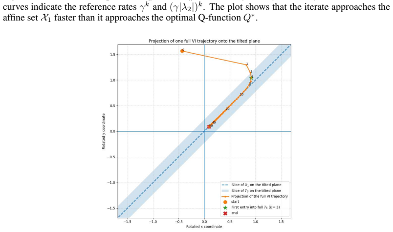
4947 17 . 5430 ] , where the (s, a )-entry represents the optimal Q-function value at state s under action a, i.e. Q∗ (s, a ). The corresponding minimum optimality gap is ∆ := min s∈S sep ¯∆ s, ¯∆ s := V ∗ (s) − max a /∈ Φ ∗ (s) Q∗ (s, a ) ≈ 0. 4022. We consider the affine space X1 = Q∗ + span(1), and choose the tube radius δ = 0 . 4∆ ≈ 0. 1609, which sati...
-
[50]
8213 17 . 8696 ] . For this particular Q0, the tie-broken greedy action is already the optimal action at every state. Thus, this single trajectory is used to visualize finite-tim e entrance into the invariant tube, rather than to demonstrate first-time policy identification from a n on-optimal greedy policy. Starting from this Q0, we run Q-VI for 50 iteratio...
-
[51]
The dotted circle indicates the boundary of the common init ial set in the (u, v )-plane
The dashed line q = p is the projection of X1, and the shaded strip is the projection of the tube Tδ, namely |q − p| ≤ 2δ. The dotted circle indicates the boundary of the common init ial set in the (u, v )-plane. Starting from 12 different initial points on this circle, the stochastic Q-l earning trajectories tend to enter the strip and then move toward t...
-
[52]
Then ¯Ai(Π ⊥ v) = λ(Π ⊥ v)
Let (v, λ ) be an eigenvector-eigenvalue pair of Ai. Then ¯Ai(Π ⊥ v) = λ(Π ⊥ v). In particular , ifΠ ⊥ v ̸= 0, then (Π ⊥ v, λ ) is an eigenvector-eigenvalue pair of ¯Ai
-
[53]
24 Proof
(1, 0) is an eigenvector-eigenvalue pair of ¯Ai. 24 Proof. Recall that ¯Ai = Π ⊥ AiΠ ⊥ , Π ⊥ = I − 1 n 11⊤ , A i1 = γ1. To prove the first statement, let (v, λ ) be an eigenvector-eigenvalue pair of Ai so that Aiv = λv . Since Π ⊥ v = v − 1⊤ v n 1, we have Ai(Π ⊥ v) = Aiv − 1⊤ v n Ai1 = λv − γ 1⊤ v n 1. Applying Π ⊥ to both sides yields ¯Ai(Π ⊥ v) = Π ⊥ Ai...
-
[54]
F or every t ≥ 0, V t+1 ε (x) ≥ ∥ x∥2 2 + β − 2 ε max i∈{ 1,...,M } V t ε ( ¯Aix)
-
[55]
F or every t ≥ 0 and every x ∈ Rn, V t ε (λx) = |λ|2V t ε (x) for all λ ∈ R, and V t ε (x) ≤ V t+1 ε (x)
-
[56]
There exists a constant Cε > 0 such that ∥x∥2 2 ≤ V t ε (x) ≤ Cε∥x∥2 2, ∀x ∈ Rn, ∀t ≥ 0
-
[57]
Moreover , ∥x∥2 2 ≤ V ∞ ε (x) ≤ Cε∥x∥2 2
F or every x ∈ Rn, the limit V ∞ ε (x) := lim t→∞ V t ε (x) exists and is finite. Moreover , ∥x∥2 2 ≤ V ∞ ε (x) ≤ Cε∥x∥2 2
-
[58]
The function pε(x) := √ V ∞ε (x) is a norm on Rn
-
[59]
The function V ∞ ε satisfies the Lyapunov inequality V ∞ ε ( ¯Aix) ≤ β 2 ε V ∞ ε (x), ∀x ∈ Rn, ∀i ∈ { 1, . . . , M }. Equivalently, pε( ¯Aix) ≤ βεpε(x), ∀x ∈ Rn, ∀i ∈ { 1, . . . , M }
-
[60]
, M }, where ∥ ¯Ai∥pε is the induced matrix norm generated by pε ∥ ¯Ai∥pε := sup x̸=0 pε( ¯Aix) pε(x)
Consequently, ∥ ¯Ai∥pε ≤ βε, ∀i ∈ { 1, . . . , M }, where ∥ ¯Ai∥pε is the induced matrix norm generated by pε ∥ ¯Ai∥pε := sup x̸=0 pε( ¯Aix) pε(x) . Therefore, we have ρ( ¯A1, ¯A2, . . . , ¯AM ) ≤ βε. Proof. We prove the statements one by one. Proof of 1). By definition, one has V t+1 ε (x) = t+1∑ k=0 β − 2k ε max ¯σ k∈{ 1,...,M } k ¯Aσ k · · ·¯Aσ 1 x ...
-
[61]
This proves 1)
For k ≥ 1, writing k = j + 1, we obtain V t+1 ε (x) = ∥x∥2 2 + t∑ j=0 β − 2(j+1) ε max ¯σ j+1 ¯Aσ j+1 · · ·¯Aσ 1 x 2 2 = ∥x∥2 2 + β − 2 ε t∑ j=0 β − 2j ε max i∈{ 1,...,M } max ¯τj∈{ 1,...,M } j ¯Aτj · · ·¯Aτ1 ¯Aix 2 2 ≥ ∥ x∥2 2 + β − 2 ε max i∈{ 1,...,M } t∑ j=0 β − 2j ε max ¯τj∈{ 1,...,M } j ¯Aτj · · ·¯Aτ1 ¯Aix 2 2 = ∥x∥2 2 + β − 2 ε...
-
[62]
By the definition of the JSR, there exists an integer K ≥ 0 such that max ¯σ k∈{ 1,...,M } k ¯Aσ k · · ·¯Aσ 1 1/k 2 ≤ η, ∀k ≥ K
For the upper bound, since ¯ρ < β ε, choose any number η such that ¯ρ < η < β ε. By the definition of the JSR, there exists an integer K ≥ 0 such that max ¯σ k∈{ 1,...,M } k ¯Aσ k · · ·¯Aσ 1 1/k 2 ≤ η, ∀k ≥ K. Hence, for all k ≥ K, we have max ¯σ k∈{ 1,...,M } k ¯Aσ k · · ·¯Aσ 1 2 ≤ ηk. Now define C0 := max { 1, max 0≤ k≤ K− 1 η− k max ¯σ k ∥...
-
[63]
Passing to the limit in the bounds of 3) yields ∥x∥2 2 ≤ V ∞ ε (x) ≤ Cε∥x∥2 2
Hence the limit V ∞ ε (x) := lim t→∞ V t ε (x) exists and is finite for every x ∈ Rn. Passing to the limit in the bounds of 3) yields ∥x∥2 2 ≤ V ∞ ε (x) ≤ Cε∥x∥2 2. Proof of 5). For each fixed k ≥ 1, define νk(x) := β − k ε max ¯σ k∈{ 1,...,M } k ∥ ¯Aσ k · · ·¯Aσ 1 x∥2. Moreover, define ν0(x) := ∥x∥2. For each k ≥ 0, νk is a seminorm, since it is the pointwis...
-
[64]
F or any ε > 0 such that βε := ¯ρ + ε < 1, there exists a constant cε > 0 such that dist2(Qk, X1) ≤ cεβ k ε dist2(Q0, X1), ∀k ≥ 0. In particular , the convergence toward the affine set X1, and hence toward the POSS X ∗ , admits exponential upper bounds at any rate larger than the J SR ¯ρ of the full restricted switching family, with the stochastic-policy c...
-
[65]
F or all k ≥ Kid, there exists a policy πk ∈ Θ ∗ such that Qk+1 − Q∗ = Aπ k (Qk − Q∗ )
-
[66]
Thus, after finite-time identification of X ∗ , the transverse component admits exponential upper bounds at any rate larger than the JSR ¯ρ∗ of the restricted optimal family
F or any ε∗ > 0 such that β∗ := ¯ρ∗ + ε∗ < 1, there exists a constant ˜Cε∗ > 0 such that ∥zKid+ℓ∥2 ≤ ˜Cε∗ β ℓ ∗ ∥zKid∥2, ∀ℓ ≥ 0. Thus, after finite-time identification of X ∗ , the transverse component admits exponential upper bounds at any rate larger than the JSR ¯ρ∗ of the restricted optimal family
-
[67]
In this case, there exists a constant Dε∗ > 0 such that ∥QKid+ℓ − Q∗ ∥2 ≤ Dε∗ γ ℓ∥QKid − Q∗∥2, ∀ℓ ≥ 0
If, in addition, ¯ρ∗ < γ , then one may choose ε∗ > 0 sufficiently small so that β∗ = ¯ρ∗ + ε∗ < γ . In this case, there exists a constant Dε∗ > 0 such that ∥QKid+ℓ − Q∗ ∥2 ≤ Dε∗ γ ℓ∥QKid − Q∗∥2, ∀ℓ ≥ 0. Proof. Write ek := Qk − Q∗ , α k := 1 n 1⊤ ek, z k := Π ⊥ ek, n := |S||A|. The global convergence estimate follows directly from Theorem 1 applied to the ...
discussion (0)
Sign in with ORCID, Apple, or X to comment. Anyone can read and Pith papers without signing in.