Program Evaluation with Remotely Sensed Outcomes
Pith reviewed 2026-05-23 17:55 UTC · model grok-4.3
The pith
A nonparametric formula identifies causal effects of programs when the outcome is measured only through remote sensing by combining experimental and observational data.
A machine-rendered reading of the paper's core claim, the machinery that carries it, and where it could break.
Core claim
Under the modeling assumption that the remotely sensed variable is caused by the economic outcome, the average treatment effect is nonparametrically identified by an explicit formula that integrates the experimental contrast in treatment assignment with the observational conditional expectation of the outcome given the remote measure; the paper supplies a corresponding estimator and inference procedure that is robust to arbitrary processing of the remote data.
What carries the argument
The nonparametric identification formula that recovers the causal parameter by combining experimental treatment assignment with the observational mapping from the remotely sensed variable to the outcome.
If this is right
- Program evaluations can use low-cost remote data for outcomes that are expensive to measure directly.
- The estimator converges at the parametric rate without parametric restrictions on how the remote data are processed.
- Inference remains valid under arbitrary misspecification of the relationship between the remote measure and the outcome.
- The approach applies to any post-outcome proxy that is predictive in observational data and observed in both experimental and observational samples.
Where Pith is reading between the lines
- The same structure could apply to other imperfect proxies such as administrative records or survey responses that are caused by the underlying outcome.
- Extensions might incorporate high-dimensional machine learning predictors for the observational mapping without changing the identification argument.
- The method could be tested in settings where both direct outcome measures and remote proxies are available in the same experiment.
Load-bearing premise
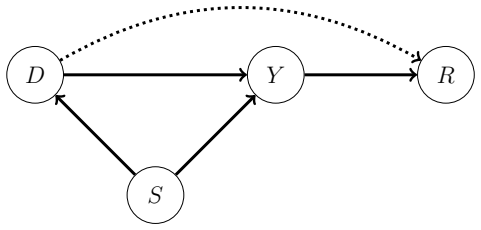
Changes in the economic outcome cause changes in the remotely sensed variable rather than the reverse.
What would settle it
An auxiliary randomized trial that directly manipulates the remotely sensed variable while holding the economic outcome fixed would produce a nonzero estimate under the identification formula if the post-outcome assumption is false.
Figures


read the original abstract
We study causal inference in experiments and quasi-experiments, where the economic outcome is imperfectly measured by a remotely sensed variable. The remotely sensed variable is low-cost, scalable, and predictive of the economic outcome in observational data; examples include satellite imagery and mobile phone activity. We model the remotely sensed variable as post-outcome: variation in the economic outcome causes variation in the remotely sensed variable. For example, changes in environmental quality cause changes in satellite imagery, not vice versa. Under this assumption, we propose a formula to nonparametrically identify the causal parameter by combining experimental and observational data. We develop a method for n^{-1/2} inference that is robust to misspecification and that does not restrict the algorithms used to process remotely sensed variables.
Editorial analysis
A structured set of objections, weighed in public.
Referee Report
Summary. The paper studies causal inference when the economic outcome of interest is imperfectly measured by a remotely sensed proxy (e.g., satellite imagery). It models the remote variable as post-outcome (outcome causes remote measure), proposes a nonparametric identification formula that fuses experimental data (treatment affects outcome and hence the remote measure) with observational data (both variables observed), and develops an n^{-1/2}-consistent inference procedure that is robust to misspecification of the remote-sensing processing algorithm.
Significance. If the identification result is valid, the approach would allow researchers to leverage low-cost, scalable remote-sensing data for program evaluation in settings where direct outcome measurement is expensive or infeasible. The robustness claim for inference is a potential strength if the conditions are fully stated.
major comments (1)
- [Abstract] Abstract: the nonparametric identification formula is stated to recover the causal parameter under the post-outcome assumption alone. However, transport of the conditional distribution P(remote | outcome) from the observational sample to the experimental sample is required for the formula to be valid; the post-outcome modeling establishes directionality but supplies no justification for invariance of this conditional law across contexts. This invariance is load-bearing for the central claim and is not addressed in the abstract.
minor comments (1)
- [Abstract] The abstract claims n^{-1/2} inference robust to misspecification without restricting the remote-sensing algorithms; the manuscript should clarify whether this robustness holds under the same invariance condition or requires additional assumptions.
Simulated Author's Rebuttal
We thank the referee for the careful reading and constructive feedback. We address the single major comment below.
read point-by-point responses
-
Referee: [Abstract] Abstract: the nonparametric identification formula is stated to recover the causal parameter under the post-outcome assumption alone. However, transport of the conditional distribution P(remote | outcome) from the observational sample to the experimental sample is required for the formula to be valid; the post-outcome modeling establishes directionality but supplies no justification for invariance of this conditional law across contexts. This invariance is load-bearing for the central claim and is not addressed in the abstract.
Authors: We agree that the abstract is imprecise on this point. The post-outcome assumption establishes the causal direction (outcome causes remote), while identification of the ATE further requires that the conditional distribution P(remote | outcome) can be transported from the observational to the experimental sample. This transportability assumption is maintained throughout the identification argument in the main text but is not mentioned in the abstract. We will revise the abstract to state the full set of assumptions under which the formula recovers the target parameter. revision: yes
Circularity Check
No circularity; identification formula is self-contained
full rationale
The paper proposes a nonparametric identification formula that fuses experimental data (treatment to outcome) with separate observational data (outcome to remote sensing) under an explicit post-outcome modeling assumption. This derivation relies on external data sources and standard causal transport arguments rather than any quantity fitted exclusively from the experimental sample, any self-citation chain, or a result defined in terms of itself. No load-bearing step reduces by construction to the inputs; the central claim retains independent content from the data combination and is therefore self-contained against external benchmarks.
Axiom & Free-Parameter Ledger
axioms (1)
- domain assumption The remotely sensed variable is post-outcome: variation in the economic outcome causes variation in the remotely sensed variable.
Forward citations
Cited by 1 Pith paper
-
Making Interpretable Discoveries from Unstructured Data: A High-Dimensional Multiple Hypothesis Testing Approach
A new framework combines AI-derived concept embeddings with high-dimensional selective inference to enable statistically principled, interpretable discovery from unstructured data in empirical economics.
Reference graph
Works this paper leans on
-
[1]
By the hypothesis that the observational sample is untreated,Pr(S = e|D = 1) = 1. Therefore, S becomes a degenerate random variable conditional uponD =1and we conclude thatS |=(Y,R)|D=1trivially
-
[2]
Weshowthat E{h(Y,R)|D =0 ,S = e}= E{h(Y,R)|D =0 ,S = o}, which impliesS |=(Y,R)|D =0as desired
Fixanybounded, measurablefunction h(Y,R). Weshowthat E{h(Y,R)|D =0 ,S = e}= E{h(Y,R)|D =0 ,S = o}, which impliesS |=(Y,R)|D =0as desired. By SUTVA, randomized treatment assignment, and randomized sample selection, E{h(Y,R)|D=0,S=e}=E[h{Y,Y R(1)+(1−Y)R(0)}|D=0,S=e] =E(h[Y(0),Y(0)R(1)+{1−Y(0)}R(0)]|D=0,S=e) =E(h[Y(0),Y(0)R(1)+{1−Y(0)}R(0)]|S=e) =E(h[Y(0),Y(...
-
[3]
To begin, we write the average potential outcome in the experimental sample as µ(1):=Pr{Y(1)=1|S=e} (1) = Pr{Y(1)=1|D=1,S=e} =Pr(Y=1|D=1,S=e) = Z Pr(Y=1|R=r,D=1,S=e)f R(r|D=1,S=e)dr, where (1) follows by Assumption 1
-
[4]
Next we rewrite the implicit target eµ(1):= Z Pr(Y=1|R=r,S=o)f R(r|D=1,S=e)dr. Within this expression, Pr(Y=1|R,S=o) (1) = fR(R|Y=1,S=o)Pr(Y=1|S=o) fR(R|S=o) (2) = fR(R|Y=1,D=1,S=e)P(Y=1|S=o) fR(R|S=o) (3) = Pr(Y=1|R,D=1,S=e) fR(R|D=1,S=e)Pr(Y=1|S=o) Pr(Y=1|D=1,S=e)f R(R|S=o) (4) = Pr(Y=1|R,D=1,S=e) Pr(Y=1|S=o) Pr{Y(1)=1|S=e} fR(R|D=1,S=e) fR(R|S=o) where...
-
[5]
Combining results, the bias for the treated potential outcome,eµ(1)−µ(1), equals Z Pr{Y(0)=1|S=e} Pr{Y(1)=1|S=e} fR(r|D=1) fR(r|D=0) −1 Pr(Y=1|R=r,D=1,S=e)f R(r|D=1,S=e)dr. Within this expression, Pr(Y=1|R,D=1,S=e)f R(R|D=1,S=e)=f Y,R(Y=1,R|D=1,S=e) =f R(R|Y=1,D=1,S=e)Pr(Y=1|D=1,S=e} =f R(R|Y=1,D=1,S=e)Pr{Y(1)=1|S=e} =f R(R|Y=1,D=1,S=e)µ(1). by the law of...
-
[6]
We can follow a similar argument foreµ(0). As in Step 2, eµ(0)= Z Pr(Y=1|R=r,S=o)f R(r|D=0,S=e)dr = Z Pr(Y=1|R=r,D=0,S=e) Pr(Y=1|S=o) Pr{Y(0)=1|S=e} fR(r|D=0,S=e) fR(r|S=o) fR(r|D=0,S=e)dr by identical arguments as before, replacingD = 1with D = 0. We have previously shown Pr(Y = 1|S = o) =Pr{Y (0) = 1|S = e}. Moreover, fR(R|D = 0,S = e) =fR(R|D = 0)since...
-
[7]
Sinceeµ(0)=µ(0), we conclude thateθ−θ=eµ(1)−µ(1)under the stated conditions
-
[8]
Suppose thatRis binary with R|Y,D,S= Ywith probability1/2 1otherwise
Next we demonstrate the bias can be positive or negative by constructing the claimed DGPs. Suppose thatRis binary with R|Y,D,S= Ywith probability1/2 1otherwise. 44 This process impliesR |=(D,S)|Y, which satisfiesR |=S|D,Y (Assumption 2) by the weak union axiom. It also directly satisfiesR |=D|Y(Assumption 3(ii)). Under this DGP, Pr(R=1|Y=1,D=1,S=e...
-
[9]
By Assumption 1,fY (y|S=e,X=x,D=d)=f Y(d) (y|S=e,X=x)
As in Lemma 1, for general(X,Y,R)and forδe d(r,x):=f R(r|S=e,X=x,D=d), δe d(r,x)= Z fR(r|S=e,X=x,D=d,Y=y)f Y (y|S=e,X=x,D=d)dy. By Assumption 1,fY (y|S=e,X=x,D=d)=f Y(d) (y|S=e,X=x). Now, however, fR(r|S=e,X=x,D=d,Y=y)=f R(r|S=o,X=x,D=d,Y=y)=:δ o y,d(r,x), where the first equality applies Assumption 2 and the second equality applies Assumption 3(i). Combi...
-
[10]
As in Theorem 1, we next apply Bayes’ rule to rewrite δo y,d(r,x)= Pr(Y=y,D=d,S=o|R=r,X=x)f R(r|X=x) Pr(Y=y,D=d,S=o|X=x) (6) δe d(r,x)= Pr(D=d,S=e|R=r,X=x)f R(r|X=x) Pr(D=d,S=e|X=x) . It therefore follows by cancelingfR(r|X=x)that, ford∈ {0,1}andr∈ R, Pr(D=d,S=e|R=r,X=x) Pr(D=d,S=e|X=x) − Pr(Y=0,D=d,S=o|R=r,X=x) Pr(Y=0,D=d,S=o|X=x) = Pr(Y=1,D=d,S=o|R=r,X=...
-
[12]
predD(R) count2 D=1,S=e + 1−pred D(R) count2 D=0,S=e # predS(R) +bθ2 init
Learn the representation ontrain:bH(R). (a) Count marginals:count Y=1,S=o,count Y=0,S=o,count D=1,S=e,count D=0,S=e. (b) Train predictors: predY (R)estimates Pr(Y = 1|S = o, R), predD(R)estimates Pr(D=1|S=e,R), andpred S(R)estimatesPr(S=e|R), using machine learning. (c) Initially estimatebθinit =argminθEtrain[{bE(∆e|R)−bE(∆o|R)θ}2], wherebE(∆e|R)and bE(∆o...
-
[13]
(a) Count marginals:count Y=1,S=o,count Y=0,S=o,count D=1,S=e,count D=0,S=e
Construct a causal estimate ontest:bθ. (a) Count marginals:count Y=1,S=o,count Y=0,S=o,count D=1,S=e,count D=0,S=e. (b) Construct a causal estimate:bθ = Etest{ b∆e bH(R)} Etest{ b∆o bH(R)} whereb∆e andb∆o are constructed from marginal probabilities according to (1): b∆e = 1{D=1,S=e} countD=1,S=e − 1{D=0,S=e} countD=0,S=e , b∆o = 1{Y=1,S=o} countY=1,S=o − ...
work page 2018
-
[14]
Divide the sample intotrainandtestfolds
-
[15]
Learn the representations ontrain:bH(R,x). For eachx∈ X, (a) Count conditional probabilities: count(D=d,S=e|X=x)= P i∈train1(Di =d,S i =e,X i =x)P i∈train1(Xi =x) for eachd∈ {0,1}, count(Y=y,S=o|X=x)= P i∈train1(Yi =y,S i =o,X i =x)P i∈train1(Xi =x) for eachy∈ Y. (b) Train predictors on the subsample withX=x: predY (R,x):R →[0,1] K using{(R i,Yi):i∈train,...
-
[16]
Construct generalized CATE estimates ontest:bθ(x). For eachx∈ X, (a) Count conditional probabilities: count(D=d,S=e|X=x)= P i∈test1(Di =d,S i =e,X i =x)P i∈test1(Xi =x) for eachd∈ {0,1}, count(Y=y,S=o|X=x)= P i∈test1(Yi =y,S i =o,X i =x)P i∈test1(Xi =x) for eachy∈ Y. (b) Compute treatment and outcome variation: b∆e(x)= 1(D=1,S=e) count(D=d,S=e|X=x) − 1(D=...
-
[17]
Aggregate into ATE estimate ontest:bθ0. (a) Compute the generalized ATE estimate:bθ=E test{bθ(X)} (b) Compute the ATE estimate:bθ0 =PK−1 j=1 yjbθj +yK 1−PK−1 j=1 bθj
-
[18]
Bootstrap its confidence interval:bθ0 ±c αbvn−1/2, where cα is the1 −α/2quantile of the standard Gaussian andbvn−1/2 is the bootstrap standard error ofbθ0 fixing the estimated representations. Our final estimatorbθ0 ∈R, for the ATE in the experimental sample, is asymptotically normal by direct extensions of the arguments in Section 4 and Appendix D. The k...
work page 2003
-
[19]
By the law of total probability and the definition of˜Yε, fR(r|S=e,X=x,D=d)= Z fR, ˜Yε(r,y|S=e,X=x,D=d)dy = Z fR(r|S=e,X=x,D=d, ˜Yε =y)f ˜Yε(y|S=e,X=x,D=d)dy = X y∈Yε fR(r|S=e,X=x,D=d, ˜Yε =y)Pr( ˜Yε =y|S=e,X=x,D=d). By the definition of˜Yε and Assumption 1, Pr( ˜Yε =y|S=e,X=x,D=d)= Z y′∈By(ε) fY (y′ |S=e,X=x,D=d)dy ′ = Z y′∈By(ε) fY(d) (y′ |S=e,X=x)dy ′ ...
-
[20]
Substituting these expressions into the previous step and cancelingfR(R|X )yields the result
We apply Bayes’ rule to rewrite fR(r|S=o,X=x, ˜Yε =y)= Pr( ˜Yε =y,S=o|R=r,X=x)f R(r|X=x) Pr( ˜Yε =y,S=o|X=x) =γ ε y(x,r)fR(r|X=x), fR(r|S=e,X=x,D=d)= Pr(D=d,S=e|R=r,X=x)f R(r|X=x) Pr(D=d,S=e|X=x) =π d(x,r)fR(r|X=x). Substituting these expressions into the previous step and cancelingfR(R|X )yields the result. Consequently,foranyfixed ε >0,wecanperformestim...
-
[21]
By equation (3), fR(r|S=e,X=x,D=d)= Z fR(r|S=o,X=x,Y=y)f Y(d) (y|S=e,X=x)dy
-
[22]
By Bayes’ rule, fR(r|Y=y,S=o,X=x)= fY,S(y,o|R=r,X=x)f R(r|X=x) fY,S(y,o|X=x) =γ 0 y(X,R)fR(r|X=x), fR(r|D=d,S=e,X=x)= Pr(D=d,S=e|R=r,X=x)f R(r|X=x) Pr(D=d,S=e|X=x) =π d(X,R)fR(r|X=x). Substituting these expressions into the previous step and cancelingfR(r|X = x)yields the result. Proposition F.3 identifies the conditional counterfactual densityfY(d) (y|S ...
work page 1989
-
[23]
By the law of total probability, δe d,i(r):=f Ri(r|S i =e,D i =d) = Z fRi,Yi(r,y|S i =e,D i =d)dy = Z fRi(r|S i =e,D i =d,Y i =y)f Yi(y|S i =e,D i =d)dy. 74 Next, notice that fRi(r|S i =e,D i =d,Y i =y)=f Ri(r|S i =o,D i =d,Y i =y) =f Ri(r|S i =o,Y i =y) =:δ o y,i(r), wherethefirstequalityappliesAssumptionI.2andthesecondequalityappliesAssumptionI.3. Combi...
-
[24]
We apply Bayes’ rule to rewrite δo y,i(r):=f Ri(r|S i =o,Y i =y)= Pr(Yi =y,S i =o|R i =r)f Ri(r) Pr(Yi =y,S i =o) , δe d,i(r):=f Ri(r|S i =e,D i =d)= Pr(Di =d,S i =e|R i =r)f Ri(r) Pr(Di =d,S i =e) . Substituting these expressions into the previous step and cancelingfRi(r)gives E(∆e i |Ri)=E(∆ o i |Ri)θi, θ i =E{Y dir i (1)−Y dir i (0)|Si =e}. We conclude...
work page 2023
-
[25]
By the law of total probability, δe d,z(r):=f R(r|S=e,D=d,Z=z) = Z fR,Y (r,y|S=e,D=d,Z=z)dy = Z fR(r|S=e,D=d,Z=z,Y=y)f Y (y|S=e,D=d,Z=z)dy. Next, notice that fR(r|S=e,D=d,Z=z,Y=y)=f R(r|S=o,D=d,Z=z,Y=y) =f R(r|S=o,Y=y) =:δ o y(r), wherethefirstequalityappliesAssumptionJ.2andthesecondequalityappliesAssumptionJ.3. 83 Combining the previous displays, we arri...
-
[26]
We apply Bayes’ rule to rewrite δo y(r):=f R(r|S=o,Y=y)= Pr(Y=y,S=o|R=r)f R(r) Pr(Y=y,S=o) , δe d,z(r):=f R(r|S=e,D=d,Z=z)= Pr(D=d,Z=z,S=e|R=r)f R(r) Pr(D=d,Z=z,S=e) . Substituting these expressions into the previous step and cancelingfR(r)yields E{∆e(d,z)−∆ oα(d,z)|R}=0. Corollary J.1(Representation with an instrument).Under Theorem J.1’s conditions, for...
work page 2023
-
[27]
By the law of total probability, δe d,t(r):=f Rt(r|S=e,D=d) = Z fRt,Yt(r,y|S=e,D=d)dy = Z fRt(r|S=e,D=d,Y t =y)f Yt(y|S=e,D=d)dy. Next, notice that fRt(r|S=e,D=d,Y t =y)=f Rt(r|S=o,D=d,Y t =y) =f Rt(r|S=o,Y t =y) =:δ o y,t(r), wherethefirstequalityappliesAssumptionJ.5andthesecondequalityappliesAssumptionJ.6. Combining the previous displays, we arrive at t...
-
[28]
We apply Bayes’ rule to rewrite δo y(r):=f Rt(r|Y t =y,S=o)= Pr(Yt =y,S=o|R t =r)f Rt(r) Pr(Yt =y,S=o) , δe d(r):=f Rt(r|D=d,S=e)= Pr(D=d,S=e|R t =r)f Rt(r) Pr(D=d,S=e) . Substituting these expressions into the previous step and cancelingfRt(r)yields E{∆e t(d)−∆ o t αt(d)|R t}=0. 86 Corollary J.2.Under Theorem J.2’s conditions, for anyt∈ {1,2}, d∈ {0,1} a...
discussion (0)
Sign in with ORCID, Apple, or X to comment. Anyone can read and Pith papers without signing in.