arxiv: 2604.19290 · v1 · submitted 2026-04-21 · 💱 q-fin.CP · q-fin.MF· q-fin.PR· q-fin.RM· stat.ME

Recognition: unknown

Orthogonal reparametrization of the Nelson-Siegel-Svensson interest rate curve model: conditioning, diagnostics, and identifiability

Daniel Guterding, Emrah G\"ulay, Robert Flassig

Authors on Pith no claims yet

Pith reviewed 2026-05-10 01:28 UTC · model grok-4.3

classification 💱 q-fin.CP q-fin.MFq-fin.PRq-fin.RMstat.ME

keywords Nelson-Siegel-Svenssonorthogonal reparametrizationQR decompositioninterest rate curvesidentifiability diagnosticsFisher information matrixyield curve fitting

0 comments

The pith

A thin QR decomposition produces orthogonal linear parameters for the Nelson-Siegel-Svensson model with a diagonal conditional Fisher information matrix.

A machine-rendered reading of the paper's core claim, the machinery that carries it, and where it could break.

The Nelson-Siegel-Svensson model for yield curves often suffers from ill-conditioning because its basis functions are nearly collinear. The paper establishes that a thin QR decomposition of the design matrix creates an orthogonal reparametrization of the linear parameters. Conditional on the nonlinear decay parameters, this makes the Fisher information matrix diagonal. This separation clarifies identifiability on the manifold where the two decay rates coincide and provides a diagnostic via the QR factor R44. In practice, it leads to smoother parameter estimates over time in Treasury data without changing the fitted curve.

Core claim

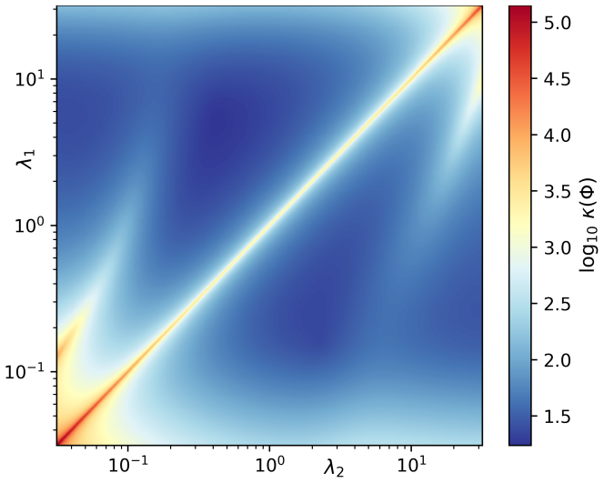
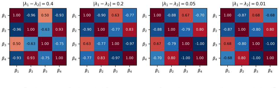
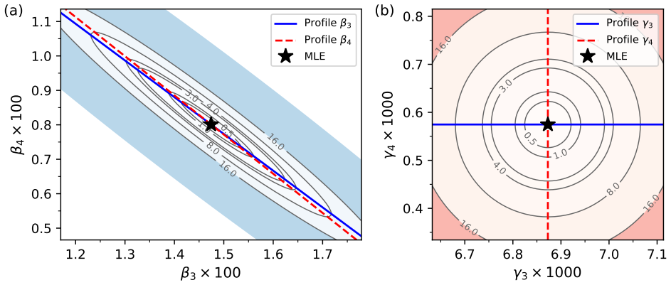
The central claim is that an exact orthogonal reparametrization via thin QR decomposition of the NSS design matrix yields orthogonal linear parameters for which the Fisher information matrix is diagonal conditional on the nonlinear parameters. A finite-horizon analytical version gives closed-form orthogonal basis entries involving exponentials, logs, and the exponential integral. Combined with Jacobian and profile-likelihood analysis, this isolates the conditioning structure from the degenerate manifold λ1=λ2 where two degrees of freedom are lost, and supplies an explicit Schur-complement covariance form for joint estimation.

What carries the argument

Thin QR decomposition applied to the NSS basis matrix, which orthogonalizes the linear parameters and diagonalizes their conditional Fisher information while preserving the original least-squares solution.

If this is right

The least-squares fit and uncertainty of the original linear parameters remain unchanged.
Full first-order covariance in orthogonal coordinates has an explicit Schur-complement form during joint nonlinear estimation of decay parameters.
Synthetic experiments confirm elimination of correlations among linear parameters and uniform conditional uncertainty.
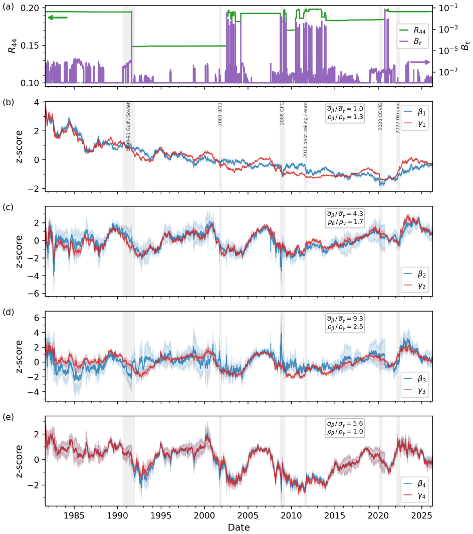
Daily U.S. Treasury analysis on fixed tenors shows smoother orthogonal parameter series than classical NSS parameters.

Where Pith is reading between the lines

These are editorial extensions of the paper, not claims the author makes directly.

The approach may extend to other separable nonlinear regression problems with collinear regressors in econometrics.
Since the moving QR basis remains nearly constant, it could enable efficient online updating of curve fits without full recomputation.
Clarifying the degenerate manifold could guide model selection between Nelson-Siegel and Svensson extensions in practice.

Load-bearing premise

The primary source of instability is collinearity in the basis functions, and the QR reparametrization fully separates this numerical issue from identifiability problems on the λ1=λ2 manifold without introducing artifacts in joint estimation.

What would settle it

If joint estimation of the decay parameters under the orthogonal coordinates still produces correlated linear parameters or non-uniform uncertainties, or if the QR basis changes substantially over time in real data, the separation of conditioning from identifiability would not hold.

Figures

Figures reproduced from arXiv: 2604.19290 by Daniel Guterding, Emrah G\"ulay, Robert Flassig.

**Figure 1.** Figure 1: Identifiability diagnostic |R44| and condition number κ(Φ) as functions of λ2 for fixed λ1 = 0.6. As λ2 → λ1, |R44| → 0 and κ → ∞. For λ2 → 0 the condition number also diverges. 0 10 20 30 Maturity (yr) 2.5 3.0 3.5 4.0 Yield (%) (a) Normal 0 10 20 30 Maturity (yr) 3.0 3.5 4.0 4.5 5.0 Yield (%) (b) Inverted 0 10 20 30 Maturity (yr) 2.0 2.5 3.0 3.5 Yield (%) (c) Humped 0 10 20 30 Maturity (yr) 2.5 3.0 3.5 4.… view at source ↗

**Figure 2.** Figure 2: Example yield curves from four synthetic regimes: (a) normal upward sloping, (b) inverted with negative initial slope, [PITH_FULL_IMAGE:figures/full_fig_p012_2.png] view at source ↗

**Figure 3.** Figure 3: Basis functions as a function of maturity for (a) the standard NSS model and (b) the discrete-QR orthogonalized [PITH_FULL_IMAGE:figures/full_fig_p014_3.png] view at source ↗

**Figure 4.** Figure 4: Condition number landscape log10 κ(Φ(λ1, λ2)) for the standard NSS basis on the finite plotting grid. The exact diagonal λ1 = λ2 and boundary singularities are excluded from the plotted finite values; analytically, κ(Φ(λ1, λ2)) diverges as these singular sets are approached. 8.3. Condition number landscape [PITH_FULL_IMAGE:figures/full_fig_p015_4.png] view at source ↗

**Figure 5.** Figure 5: Correlation matrices for the standard β parametrization across four conditioning regimes. The maximum absolute offdiagonal correlation reported in [PITH_FULL_IMAGE:figures/full_fig_p016_5.png] view at source ↗

**Figure 6.** Figure 6: Profile negative log-likelihood ∆NLL for the four linear parameters: level (β1/γ1), slope (β2/γ2), curvature (β3/γ3), and second hump (β4/γ4). Blue solid: standard βj ; red dashed: orthogonal γj . (a-d) well-separated case (λ1 = 0.6, λ2 = 0.2). (e-h) very degenerate case (λ1 = 0.6, λ2 = 0.59). The x-axis shows (θj − θˆ j )/σ so both parametrizations share the same scale; the grey horizontal line marks the … view at source ↗

**Figure 7.** Figure 7: Two-dimensional ∆NLL landscape over parameter pairs (β3, β4) (a) and (γ3, γ4) (b) in the well-separated regime (λ1 = 0.6, λ2 = 0.4). Contour labels show ∆NLL values; the 3.0 contour corresponds to the joint 95% confidence region ( 1 2 χ 2 2,0.95 ≈ 3.0). Profile paths (solid: parameter 3 profiled; dashed: parameter 4 profiled) show the optimizer’s trajectory when fixing one parameter and optimizing the rest… view at source ↗

**Figure 8.** Figure 8: Daily US Treasury application on the fixed reduced 9-tenor grid. (a, b) aggregate stability diagnostics for the classical [PITH_FULL_IMAGE:figures/full_fig_p020_8.png] view at source ↗

**Figure 9.** Figure 9: Daily identifiability and long-run state representation on the fixed reduced 9-tenor grid (1981–2026). (a) the iden [PITH_FULL_IMAGE:figures/full_fig_p021_9.png] view at source ↗

**Figure 10.** Figure 10: Exact monthly changepoint analysis on the fixed reduced 9-tenor grid. (a) exact dynamic-programming cost paths [PITH_FULL_IMAGE:figures/full_fig_p022_10.png] view at source ↗

read the original abstract

The Nelson-Siegel-Svensson (NSS) interest rate curve model yields a separable nonlinear least-squares problem whose inner linear block is often ill-conditioned because the basis functions become nearly collinear. We analyze this instability via an exact orthogonal reparametrization of the design matrix. A thin QR decomposition produces orthogonal linear parameters for which, conditional on the nonlinear parameters, the Fisher information matrix is diagonal. We also derive a finite-horizon analytical orthogonalization: on $[0,T]$, the $4\times 4$ continuous Gram matrix has closed-form entries involving exponentials, logarithms, and the exponential integral $E_1$, yielding an explicit horizon-dependent orthogonal NSS basis. Together with Jacobian-rank and profile-likelihood arguments, this representation clarifies the degenerate manifold $\lambda_1=\lambda_2$, where the Svensson extension loses two degrees of freedom. Orthogonalization leaves the least-squares fit and uncertainty of the original linear parameters unchanged, but isolates the conditioning structure. When the decay parameters are estimated jointly, the full first-order covariance in orthogonal coordinates admits an explicit Schur-complement form. The approach also yields a scalar identifiability diagnostic through the QR element $R_{44}$ and separates model reduction from numerical instability. Synthetic experiments confirm that orthogonal parametrization eliminates correlations among the linear parameters and keeps their conditional uncertainty uniform. A daily U.S. Treasury study on a reduced fixed 9-tenor grid from 1981 to 2026 shows smoother orthogonal parameter series than classical NSS parameters while the moving QR basis remains nearly constant.

Editorial analysis

A structured set of objections, weighed in public.

Desk editor's note, referee report, simulated authors' rebuttal, and a circularity audit. Tearing a paper down is the easy half of reading it; the pith above is the substance, this is the friction.

Desk Editor's Note private letter to a colleague

The paper gives a QR-based orthogonal reparametrization for the NSS yield curve that diagonalizes the conditional Fisher information and flags the λ1=λ2 degeneracy with the R44 entry.

read the letter

The main point is that the authors apply a thin QR factorization to the NSS design matrix, conditional on the nonlinear decay parameters. This produces an orthogonal basis for the linear coefficients, so their conditional Gram matrix is the identity and the Fisher information is diagonal by construction. They also derive the exact 4x4 continuous Gram matrix on [0,T] whose entries involve exponentials, logs, and the exponential integral E1, giving an explicit horizon-dependent orthogonal NSS basis. The R44 element from the QR serves as a scalar check for the rank drop when λ1 equals λ2, consistent with the Jacobian and profile-likelihood analysis they reference. The reparametrization is an equivalence transform, so fitted values and original-parameter uncertainties stay the same while the numerics improve. Synthetic runs show the linear-parameter correlations vanish and conditional variances become uniform. The U.S. Treasury example on the fixed 9-tenor grid produces smoother orthogonal-parameter paths than the classical ones, with the moving basis staying nearly constant. This is useful because it separates numerical conditioning from the identifiability problem on the degenerate manifold without adding artifacts. The Schur-complement form for the joint covariance follows directly from the same orthogonalization. The derivations are algebraic and standard once the QR step is taken, so the claims hold up on their own terms. The main limitation is that the Treasury study uses a reduced tenor grid, which may understate how the method behaves on denser market data. They do not release code or full numerical error analysis for the closed-form E1 expressions, but the underlying linear algebra is reproducible. This work is aimed at practitioners who estimate parametric yield curves daily and run into collinearity in the linear block. A reader who fits NSS or similar separable nonlinear models in fixed income will find the explicit formulas and the R44 diagnostic immediately usable. It deserves a serious referee because the technique is clean, the experiments are confirmatory rather than overstated, and the identifiability clarification is concrete. I would send it out for review.

Referee Report

0 major / 4 minor

Summary. The manuscript proposes an orthogonal reparametrization of the Nelson-Siegel-Svensson (NSS) model via thin QR factorization of the design matrix (conditional on the nonlinear decay parameters) to resolve ill-conditioning from near-collinear basis functions. It derives a closed-form 4×4 continuous Gram matrix on [0,T] whose entries involve exponentials, logarithms, and the exponential integral E1, yielding an explicit horizon-dependent orthogonal basis. The approach supplies a scalar identifiability diagnostic (vanishing R44 on the λ1=λ2 manifold), an explicit Schur-complement expression for the joint covariance, and separates numerical conditioning from identifiability loss. Synthetic experiments and a daily U.S. Treasury study on a fixed 9-tenor grid (1981–2026) are used to illustrate that the reparametrized linear parameters exhibit zero conditional correlation, uniform uncertainty, and smoother time series while preserving the original fit and uncertainties.

Significance. If the algebraic derivations hold, the work supplies a practical, equivalence-preserving transformation that directly diagonalizes the conditional Fisher information for the linear block of NSS models, a widely used tool in fixed-income analytics. The closed-form orthogonal basis and R44 diagnostic offer concrete tools for both numerical stability and model-reduction decisions. The separation of conditioning artifacts from the genuine two-degree-of-freedom loss on λ1=λ2 is a useful clarification. The explicit Schur-complement covariance and reproducible synthetic/real-data illustrations are strengths that could improve the reliability of joint nonlinear estimation routines.

minor comments (4)

[Abstract] Abstract: the statement that 'the moving QR basis remains nearly constant' is presented without a quantitative summary statistic (e.g., average Frobenius norm of day-to-day differences in the Q factor or condition-number trajectory); adding such a metric would strengthen the empirical claim.
The continuous Gram-matrix derivation is asserted to be closed-form, yet the manuscript does not indicate whether the explicit expressions for the four diagonal and six off-diagonal entries (involving E1) are collected in an appendix or supplementary file; providing them would aid verification and implementation.
Notation: the orthogonal linear parameters are referred to interchangeably as 'transformed' and 'orthogonal' without a single consistent symbol (e.g., β⊥ or βQR); introducing and using one symbol throughout would reduce reader confusion when comparing conditional covariances.
The profile-likelihood and Jacobian-rank arguments for the λ1=λ2 degeneracy are invoked but not cross-referenced to the R44 diagnostic in a single location; a short dedicated subsection linking the three approaches would clarify their equivalence.

Simulated Author's Rebuttal

0 responses · 0 unresolved

We thank the referee for the positive and accurate summary of our manuscript, which correctly highlights the QR orthogonal reparametrization, the closed-form continuous Gram matrix on [0,T], the R44 identifiability diagnostic, and the separation of conditioning from the λ1=λ2 degeneracy. The recommendation for minor revision is noted. As no specific major comments were provided, we have no points requiring response or revision.

Circularity Check

0 steps flagged

No significant circularity: reparametrization follows standard QR algebra

full rationale

The paper applies the thin QR factorization to the NSS design matrix conditional on the nonlinear parameters, which by the algebraic definition of the orthonormal Q factor produces a diagonal conditional Gram matrix (and thus Fisher information) without any fitted quantities or self-referential definitions. This is an equivalence transformation that preserves the original fit and uncertainties, and the identifiability diagnostics (R44 vanishing on λ1=λ2, Schur-complement covariance, closed-form continuous Gram matrix with E1) are direct consequences of the same orthogonalization plus standard Jacobian-rank and profile-likelihood arguments. No step reduces a claimed prediction or uniqueness result to its own inputs by construction, and there are no load-bearing self-citations or ansatzes smuggled in. The derivation is self-contained against external linear-algebra benchmarks.

Axiom & Free-Parameter Ledger

0 free parameters · 2 axioms · 0 invented entities

The work rests on standard linear-algebra facts and the conventional functional form of the NSS model; no new free parameters, axioms beyond basic mathematics, or invented entities are introduced.

axioms (2)

standard math Thin QR decomposition exists and is unique up to sign for a full-column-rank design matrix
Invoked to obtain orthogonal linear parameters
domain assumption The NSS basis functions are the standard exponential forms with two decay rates
Taken as given from the established model

pith-pipeline@v0.9.0 · 5614 in / 1338 out tokens · 37769 ms · 2026-05-10T01:28:35.363304+00:00 · methodology

discussion (0)

Reference graph

Works this paper leans on

45 extracted references · 39 canonical work pages

[1]

Waggoner

D.F. Waggoner. Spline methods for extracting interest rate curves from coupon bond prices.Federal Reserve Bank of Atlanta Working Paper, No. 97–10, 1997

1997
[2]

Parsimoniousmodelingofyieldcurves.Journal of Business, 60(4):473–489,

C.R.NelsonandA.F.Siegel. Parsimoniousmodelingofyieldcurves.Journal of Business, 60(4):473–489,
[3]

Svensson

L.E.O. Svensson. Estimating and interpreting forward interest rates: Sweden 1992–1994.IMF Working Paper, WP/94/114, 1994

1992
[4]

Zero-coupon yield curves: Technical documentation.BIS Papers, No

Bank for International Settlements. Zero-coupon yield curves: Technical documentation.BIS Papers, No. 25, 2005

2005
[5]

Gürkaynak and Brian Sack and Jonathan H

R.S. Gürkaynak, B. Sack, and J.H. Wright. The U.S. Treasury yield curve: 1961 to the present.Journal of Monetary Economics, 54(8):2291–2304, 2007. doi:10.1016/j.jmoneco.2007.06.029

work page doi:10.1016/j.jmoneco.2007.06.029 1961
[6]

Diebold and G.S

F.X. Diebold and G.S. Rudebusch.Yield Curve Modeling and Forecasting: The Dynamic Nelson–Siegel Approach. Princeton University Press, 2013. doi:10.1515/9781400845415

work page doi:10.1515/9781400845415 2013
[7]

Diebold and C

F.X. Diebold and C. Li. Forecasting the term structure of government bond yields.Journal of Econo- metrics, 130(2):337–364, 2006. doi:10.1016/j.jeconom.2005.03.005

work page doi:10.1016/j.jeconom.2005.03.005 2006
[8]

Gauthier and J.-G

G. Gauthier and J.-G. Simonato. Linearized Nelson–Siegel and Svensson models for the esti- mation of spot interest rates.European Journal of Operational Research, 219(2):442–451, 2012. doi:10.1016/j.ejor.2012.01.004

work page doi:10.1016/j.ejor.2012.01.004 2012
[9]

Gimeno and J.M

R. Gimeno and J.M. Nave. A genetic algorithm estimation of the term structure of interest rates. Computational Statistics & Data Analysis, 53(6):2236–2250, 2009. doi:10.1016/j.csda.2008.10.030

work page doi:10.1016/j.csda.2008.10.030 2009
[10]

Annaert, A.G.P

J. Annaert, A.G.P. Claes, M.J.K. De Ceuster, and H. Zhang. Estimating the spot rate curve using the Nelson–Siegel model: A ridge regression approach.International Review of Economics & Finance, 27:482–496, 2013. doi:10.1016/j.iref.2013.01.005

work page doi:10.1016/j.iref.2013.01.005 2013
[11]

Optimization

D. Banholzer, J. Fliege, and R. Werner. Revisiting the fitting of the Nelson–Siegel and Svensson models. Optimization, 73(10):3021–3053, 2024. doi:10.1080/02331934.2024.2389242. 26

work page doi:10.1080/02331934.2024.2389242 2024
[12]

De Pooter

M. De Pooter. Examining the Nelson–Siegel class of term structure models.Tinbergen Institute Dis- cussion Paper, No. 2007-043/4, 2007

2007
[13]

Hoerl and Robert W

A.E. Hoerl and R.W. Kennard. Ridge regression: Biased estimation for nonorthogonal problems. Technometrics, 12(1):55–67, 1970. doi:10.1080/00401706.1970.10488634

work page doi:10.1080/00401706.1970.10488634 1970
[14]

Bolder and D

D.J. Bolder and D. Stréliski. Yield curve modelling at the Bank of Canada.Bank of Canada Technical Report, No. 84, 1999. doi:10.34989/tr-84

work page doi:10.34989/tr-84 1999
[15]

Gilli, S

M. Gilli, S. Große, and E. Schumann. Calibrating the Nelson–Siegel–Svensson model.COMISEF Working Paper Series, No. WPS-031, 2010

2010
[16]

Belsley, E

D.A. Belsley, E. Kuh, and R.E. Welsch.Regression Diagnostics: Identifying Influential Data and Sources of Collinearity. Wiley, New York, 1980. doi:10.1002/0471725153

work page doi:10.1002/0471725153 1980
[17]

Golub and Victor Pereyra

G.H. Golub and V. Pereyra. The differentiation of pseudo-inverses and nonlinear least squares problems whose variables separate.SIAM Journal on Numerical Analysis, 10(2):413–432, 1973. doi:10.1137/0710036

work page doi:10.1137/0710036 1973
[18]

Golub and V

G.H. Golub and V. Pereyra. Separable nonlinear least squares: The variable projection method and its applications.Inverse Problems, 19(2):R1–R26, 2003. doi:10.1088/0266-5611/19/2/201

work page doi:10.1088/0266-5611/19/2/201 2003
[19]

Ruhe and P.-Å

A. Ruhe and P.-Å. Wedin. Algorithms for separable nonlinear least squares problems.SIAM Review, 22(3):318–337, 1980. doi:10.1137/1022057

work page doi:10.1137/1022057 1980
[20]

L. Kaufman. A variable projection method for solving separable nonlinear least squares problems.BIT Numerical Mathematics, 15(1):49–57, 1975. doi:10.1007/BF01932995

work page doi:10.1007/bf01932995 1975
[21]

O’Leary and B.W

D.P. O’Leary and B.W. Rust. Variable projection for nonlinear least squares problems.Computational Optimization and Applications, 54(3):579–593, 2013. doi:10.1007/s10589-012-9492-9

work page doi:10.1007/s10589-012-9492-9 2013
[22]

Cox and N

D.R. Cox and N. Reid. Parameter orthogonality and approximate conditional inference.Journal of the Royal Statistical Society: Series B, 49(1):1–18, 1987. doi:10.1111/j.2517-6161.1987.tb01422.x

work page doi:10.1111/j.2517-6161.1987.tb01422.x 1987
[23]

Guterding

D. Guterding. Sparse modeling approach to the arbitrage-free interpolation of plain-vanilla option prices and implied volatilities.Risks, 11(5):83, 2023. doi:10.3390/risks11050083

work page doi:10.3390/risks11050083 2023
[24]

Stewart.Matrix Algorithms, Volume 1: Basic Decompositions

G.W. Stewart.Matrix Algorithms, Volume 1: Basic Decompositions. SIAM, Philadelphia, 1998. doi:10.1137/1.9781611971408

work page doi:10.1137/1.9781611971408 1998
[25]

Melnichenko, R

M. Melnichenko, R. Murray, W. Killian, J. Demmel, M.W. Mahoney, P. Luszczek, and M. Gates. Anatomy of high-performance column-pivoted QR decomposition. arXiv preprint arXiv:2507.00976,

work page arXiv
[26]

doi:10.48550/arXiv.2507.00976

work page doi:10.48550/arxiv.2507.00976
[27]

Accuracy and Stability of Numerical Algorithms (2nd ed.)

N.J. Higham.Accuracy and Stability of Numerical Algorithms. SIAM, Philadelphia, 2nd edition, 2002. doi:10.1137/1.9780898718027

work page doi:10.1137/1.9780898718027 2002
[28]

Rothenberg

T.J. Rothenberg. Identification in parametric models.Econometrica, 39(3):577–591, 1971. doi:10.2307/1913267

work page doi:10.2307/1913267 1971
[29]

Ljung and S.T

L. Ljung and S.T. Glad. On global identifiability for arbitrary model parametrizations.Automatica, 30(2):265–276, 1994. doi:10.1016/0005-1098(94)90029-9

work page doi:10.1016/0005-1098(94)90029-9 1994
[30]

Catchpole and B.J.T

E.A. Catchpole and B.J.T. Morgan. Detecting parameter redundancy.Biometrika, 84(1):187–196, 1997. doi:10.1093/biomet/84.1.187

work page doi:10.1093/biomet/84.1.187 1997
[31]

A. Raue, C. Kreutz, T. Maiwald, J. Bachmann, M. Schilling, U. Klingmüller, and J. Timmer. Structural and practical identifiability analysis of partially observed dynamical models by exploiting the profile likelihood.Bioinformatics, 25(15):1923–1929, 2009. doi:10.1093/bioinformatics/btp358. 27

work page doi:10.1093/bioinformatics/btp358 1923
[32]

Profile-Wise Analysis: A profile likelihood-based workflow for identifiability analysis, estimation, and prediction with mechanis- tic mathematical models

M.J. Simpson and O.J. Maclaren. Profile-Wise Analysis: A profile likelihood-based workflow for iden- tifiability analysis, estimation, and prediction with mechanistic mathematical models.PLOS Compu- tational Biology, 19(9):e1011515, 2023. doi:10.1371/journal.pcbi.1011515

work page doi:10.1371/journal.pcbi.1011515 2023
[33]

The strong coupling constant: state of the art and the decade ahead,

M.I. Español and M. Pasha. Variable projection methods for separable nonlinear inverse problems with general-form Tikhonov regularization.Inverse Problems, 39(8):084002, 2023. doi:10.1088/1361- 6420/acdd1b

work page doi:10.1088/1361- 2023
[34]

Comerso Salzer, M.I

D.B. Comerso Salzer, M.I. Español, and G. Jeronimo. Variable projection methods for solving reg- ularized separable inverse problems with applications to semi-blind image deblurring. arXiv preprint arXiv:2601.05224, 2026. doi:10.48550/arXiv.2601.05224

work page doi:10.48550/arxiv.2601.05224 2026
[35]

Español and G

M.I. Español and G. Jeronimo. Local convergence analysis of a variable projection method for reg- ularized separable nonlinear inverse problems.SIAM J. Matrix Anal. Appl., 46(2):858–878, 2025. doi:10.1137/24M1639087

work page doi:10.1137/24m1639087 2025
[36]

A comparison of three methods for selecting values of input variables in the analysis of output from a computer code.Technometrics1979, 21, 239–245

G.H. Golub, M. Heath, and G. Wahba. Generalized cross-validation as a method for choosing a good ridge parameter.Technometrics, 21(2):215–223, 1979. doi:10.1080/00401706.1979.10489751

work page doi:10.1080/00401706.1979.10489751 1979
[37]

Bellec, J.-H

P.C. Bellec, J.-H. Du, T. Koriyama, P. Patil, and K. Tan. Corrected generalized cross-validation for finite ensembles of penalized estimators.J. R. Stat. Soc. Ser. B Stat. Methodol., 87(2):289–318, 2025. doi:10.1093/jrsssb/qkae092

work page doi:10.1093/jrsssb/qkae092 2025
[38]

P.C. Hansen. Analysis of discrete ill-posed problems by means of the L-curve.SIAM Review, 34(4):561– 580, 1992. doi:10.1137/1034115

work page doi:10.1137/1034115 1992
[39]

Campbell, C

S.D. Campbell, C. Li, and J. Im. Measuring agency MBS market liquidity with transaction data.FEDS Notes, Board of Governors of the Federal Reserve System, 2014. doi:10.17016/2380-7172.0007

work page doi:10.17016/2380-7172.0007 2014
[40]

Björck.Numerical Methods for Least Squares Problems

Å. Björck.Numerical Methods for Least Squares Problems. SIAM, Philadelphia, 1996. doi:10.1137/1.9781611971484

work page doi:10.1137/1.9781611971484 1996
[41]

Litterman and J

R. Litterman and J. Scheinkman. Common factors affecting bond returns.Journal of Fixed Income, 1(1):54–61, 1991. doi:10.3905/jfi.1991.692347

work page doi:10.3905/jfi.1991.692347 1991
[42]

Guterding and W

D. Guterding and W. Boenkost. The Heston stochastic volatility model with piecewise constant pa- rameters: efficient calibration and pricing of window barrier options.Journal of Computational and Applied Mathematics, 343:353–362, 2018. doi:10.1016/j.cam.2018.04.054

work page doi:10.1016/j.cam.2018.04.054 2018
[43]

Christensen, F.X

J.H.E. Christensen, F.X. Diebold, and G.D. Rudebusch. The affine arbitrage-free class of Nelson–Siegel term structure models.Journal of Econometrics, 164(1):4–20, 2011. doi:10.1016/j.jeconom.2011.02.011

work page doi:10.1016/j.jeconom.2011.02.011 2011
[44]

Caldeira, W.C

J.F. Caldeira, W.C. Cordeiro, E. Ruiz, and A.A.P. Santos. Forecasting the yield curve: the role of additional and time-varying decay parameters, conditional heteroscedasticity, and macro-economic factors.J. Time Ser. Anal., 46(2):258–285, 2025. doi:10.1111/jtsa.12769

work page doi:10.1111/jtsa.12769 2025
[45]

Resnik and M

D.B. Resnik and M. Hosseini. Disclosing artificial intelligence use in scientific research and publica- tion: When should disclosure be mandatory, optional, or unnecessary?Accountability in Research, 33(2):2481949, 2026. doi:10.1080/08989621.2025.2481949. 28

work page doi:10.1080/08989621.2025.2481949 2026