Transformers Can Learn Posterior Predictive Distributions In-Context
Pith reviewed 2026-06-29 16:02 UTC · model grok-4.3
The pith
Transformers can implement gradient descent to approximate posterior predictive distributions of Gaussian processes.
A machine-rendered reading of the paper's core claim, the machinery that carries it, and where it could break.
Core claim
By explicit construction, a transformer can realize a gradient descent algorithm that targets the posterior predictive mean and variance for Gaussian process regression. Nonlinear mappings then turn these quantities into binned probabilities that approximate the full posterior predictive distribution. The analysis provides error bounds in terms of the number of attention layers and the fineness of the probability bins, and identifies normalization as essential for extrapolation outside the pretraining range.
What carries the argument
Gradient descent steps on the Gaussian process posterior mean and variance implemented by transformer attention, combined with nonlinear mappings to produce binned PPD probabilities.
If this is right
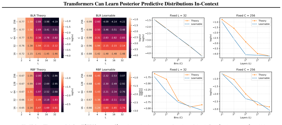
- The approximation error of the PPD decreases with greater attention depth and finer bin resolution.
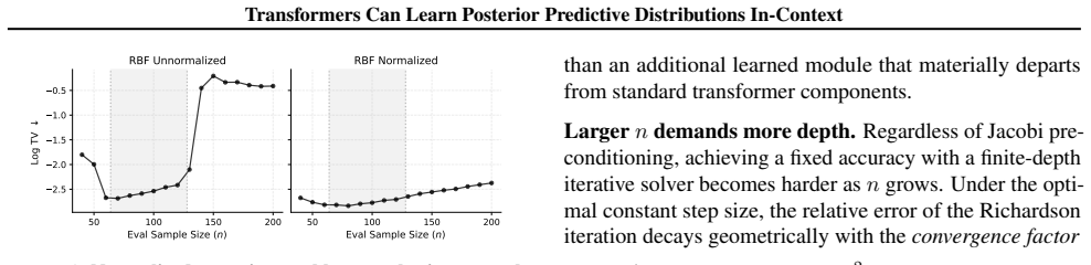
- Normalization is required for the transformer to extrapolate its PPD estimates beyond the sample sizes seen in pretraining.
- Attention depth directly governs how accurately the model can perform in-context Bayesian prediction.
- Transformers of this form can supply full distributional outputs rather than point predictions alone.
Where Pith is reading between the lines
- Analogous constructions could embed gradient updates for other Bayesian models inside attention layers.
- Attention depth may serve as a general control on accuracy across a broader set of in-context learning problems.
- Bin resolution can be chosen in practice to match the precision needed for downstream probability estimates.
- The approach may encounter limits when data-generating processes depart from Gaussian process assumptions.
Load-bearing premise
The transformer architecture with normalization is sufficient to realize the exact gradient descent steps on the Gaussian-process posterior mean and variance without additional fitting.
What would settle it
A trained transformer on Gaussian process regression tasks produces binned probabilities that deviate from the true posterior predictive distribution even when attention depth is increased, or extrapolation fails once normalization is removed.
Figures

read the original abstract
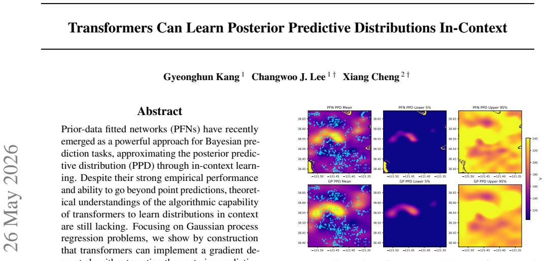
Prior-data fitted networks (PFNs) have recently emerged as a powerful approach for Bayesian prediction tasks, approximating the posterior predictive distribution (PPD) through in-context learning. Despite their strong empirical performance and ability to go beyond point predictions, theoretical understandings of the algorithmic capability of transformers to learn distributions in context are still lacking. Focusing on Gaussian process regression problems, we show by construction that transformers can implement a gradient descent algorithm targeting the posterior predictive mean and variance, followed by nonlinear mappings that yield binned probabilities of PPD. We study the error bounds of the approximated PPD in terms of attention depth and bin resolution. Based on these results, we further demonstrate the key role of normalization and the choice of attention depth in enabling the extrapolation abilities of transformers beyond the pretraining sample size range. We conduct simulations that corroborate our findings, providing insight into the expressivity of PFNs targeting PPDs and how architectural choices may influence generalization capabilities.
Editorial analysis
A structured set of objections, weighed in public.
Referee Report
Summary. The paper claims to show by construction that transformers can implement a finite-step gradient descent algorithm targeting the posterior predictive mean and variance for Gaussian process regression, followed by fixed nonlinear mappings to produce binned probabilities of the PPD. Error bounds are stated in terms of attention depth and bin resolution. The work further identifies the key role of normalization (and attention depth) in enabling extrapolation beyond the pretraining sample-size range, with simulations reported to corroborate both the construction and the extrapolation behavior.
Significance. If the explicit construction holds, the result supplies a concrete theoretical account of how transformers can realize Bayesian posterior predictive inference in-context, directly explaining the empirical success of prior-data fitted networks on distribution-valued tasks. The error analysis, the isolation of normalization as the mechanism for out-of-range generalization, and the provision of simulation evidence constitute clear strengths for a manuscript in this area.
minor comments (3)
- [Construction section] The abstract and introduction refer to 'the specific transformer architecture (including normalization)' but do not list the precise layer-norm placement or scaling constants used in the construction; this should be stated explicitly in the section presenting the weight construction.
- [Simulations] In the simulation section, the reported figures compare in-context performance inside versus outside the pretraining length range, but the exact bin resolution and number of GD steps used for each curve are not tabulated; adding a small table would improve reproducibility.
- [Error analysis] The error-bound statements are given in terms of depth and bin resolution, yet the dependence on the GP kernel hyperparameters is left implicit; a short remark clarifying whether the bounds are uniform over a compact set of kernels would be helpful.
Simulated Author's Rebuttal
We thank the referee for the positive assessment of our work and the recommendation of minor revision. The provided summary accurately captures the paper's construction of transformers implementing finite-step gradient descent on posterior predictive mean and variance for Gaussian process regression, followed by binning, along with the error analysis and the role of normalization in extrapolation.
Circularity Check
No significant circularity: constructive existence result with independent verification steps
full rationale
The paper's central claim is an explicit construction showing that a specific transformer architecture (with normalization) can realize finite-step gradient descent on the GP posterior mean and variance, followed by fixed nonlinear maps to binned PPD probabilities. Error bounds are derived in terms of depth and bin resolution; simulations corroborate both the construction and the role of normalization. No load-bearing step reduces by definition to a fitted parameter, no self-citation chain is invoked to justify the core mapping, and the derivation does not rename or smuggle in prior results from the same authors. The result is therefore self-contained against external benchmarks and receives the default non-circularity finding.
Axiom & Free-Parameter Ledger
Reference graph
Works this paper leans on
-
[1]
Brown, T., Mann, B., Ryder, N., Subbiah, M., Kaplan, J
ISBN 9780199535255. Brown, T., Mann, B., Ryder, N., Subbiah, M., Kaplan, J. D., Dhariwal, P., Neelakantan, A., Shyam, P., Sastry, G., Askell, A., Agarwal, S., Herbert-V oss, A., Krueger, G., Henighan, T., Child, R., Ramesh, A., Ziegler, D., Wu, J., Winter, C., Hesse, C., Chen, M., Sigler, E., Litwin, M., Gray, S., Chess, B., Clark, J., Berner, C., McCandl...
1901
-
[2]
A survey on in-context learning
Dong, Q., Li, L., Dai, D., Zheng, C., Ma, J., Li, R., Xia, H., Xu, J., Wu, Z., Chang, B., Sun, X., Li, L., and Sui, Z. A survey on in-context learning. In Al-Onaizan, Y ., Bansal, M., and Chen, Y .-N. (eds.),Proceedings of the 2024 Conference on Empirical Methods in Natural Lan- guage Processing, pp. 1107–1128, Miami, Florida, USA, November
2024
-
[3]
TabPFN-2.5: Advancing the State of the Art in Tabular Foundation Models
10 Transformers Can Learn Posterior Predictive Distributions In-Context Grinsztajn, L., Fl¨oge, K., Key, O., Birkel, F., Jund, P., Roof, B., J¨ager, B., Safaric, D., Alessi, S., Hayler, A., Manium, M., Yu, R., Jablonski, F., Hoo, S. B., Garg, A., Robertson, J., B ¨uhler, M., Moroshan, V ., Purucker, L., Cornu, C., Wehrhahn, L. C., Bonetto, A., Sch ¨olkopf...
work page internal anchor Pith review Pith/arXiv arXiv
-
[4]
Grinsztajn, L., Fl¨oge, K., Key, O., Birkel, F., Jund, P., Roof, B., Manium, M., Bin, S., Hoo, B ¨uhler, M., Garg, A., Safaric, D., Robertson, J., J¨ager, B., Alessi, S., Hayler, A., Moroshan, V ., Purucker, L., Singer, P., Arazi, A., Siems, J., Metzen, J. H., Grab, G., Erickson, N., Guo, S., Kalfon, E., Bing, S., Salinas, D., Cornu, C., Wehrhahn, L. C., ...
work page internal anchor Pith review Pith/arXiv arXiv
-
[5]
P., and Sesh Kumar, K
Moriconi, R., Deisenroth, M. P., and Sesh Kumar, K. High-dimensional Bayesian optimization using low- dimensional feature spaces.Machine Learning, 109(9): 1925–1943,
1925
-
[6]
Tabpfn: One model to rule them all?arXiv preprint arXiv:2505.20003, 2025
Zhang, Q., Tan, Y . S., Tian, Q., and Li, P. TabPFN: One model to rule them all?arXiv preprint arXiv:2505.20003,
-
[7]
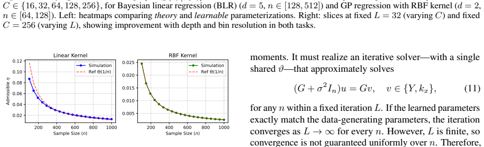
Hence, the above quantities can be expressed in terms ofλ j(D−1/2AD−1/2),j∈ {1, n}as well
Note that D−1A and D−1/2AD−1/2 are similar matrices, so they have the same characteristic polynomials, hence the same eigenvalues. Hence, the above quantities can be expressed in terms ofλ j(D−1/2AD−1/2),j∈ {1, n}as well. B. Auxiliary Lemmas and Theorems B.1. Approximation based on Discretization Lemma B.1.Let p(x) be a LLip-Lipschitz continuous density s...
2013
-
[8]
-st (hence smallest) sample eigenvalues is upper bounded through trace bounds and Markov inequality, following the technique in Burt et al. (2019). Let κ(x, x′) = exp −0.5∥x−x ′∥2 be the RBF kernel. By Mercer’s theorem, the spectral decomposition is κ(x, x′) =P j≥1 µjϕj(x)ϕj(x′)where{ϕ j}are orthonormal basis and{µ j}are eigenvalues. The largest eigenvalu...
2019
-
[9]
Fix a compact set K ⊂R×(0,∞) on which the mapping ψ:K →R 2 is defined as ψ: (µ, τ)7→ µ τ ,− 1 2τ
the target PPD belongs to a one-dimensional exponential familyf θ(y), 3.f θ(y)is Lipschitz continuous on(a, b]and the grid is equidistant. Fix a compact set K ⊂R×(0,∞) on which the mapping ψ:K →R 2 is defined as ψ: (µ, τ)7→ µ τ ,− 1 2τ . Such K is plausible given that y∈(a, b] and τ(Z (0))∈[σ 2, σ2 +κ(x, x)] for any Z(0). By the universal approximation th...
1991
-
[10]
Task FigureLR base N BLR (theory), trainTF ϑ,L Fig
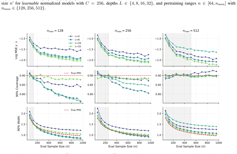
All the metrics in the figures are evaluated on4096evaluation samples. Task FigureLR base N BLR (theory), trainTF ϑ,L Fig. 22×10 −4 104 BLR (learnable), trainTF ϑ,L Fig. 22×10 −4 2×10 4 RBF (theory), trainTF ϑ,L Fig. 21×10 −3 5×10 4 RBF (learnable), trainTF ϑ,L Fig. 22×10 −4 105 RBF (learnable), trainTF ϑ,L Fig. 42×10 −4 105 RBF (learnable), trainTF pr ϑ,...
2007
-
[11]
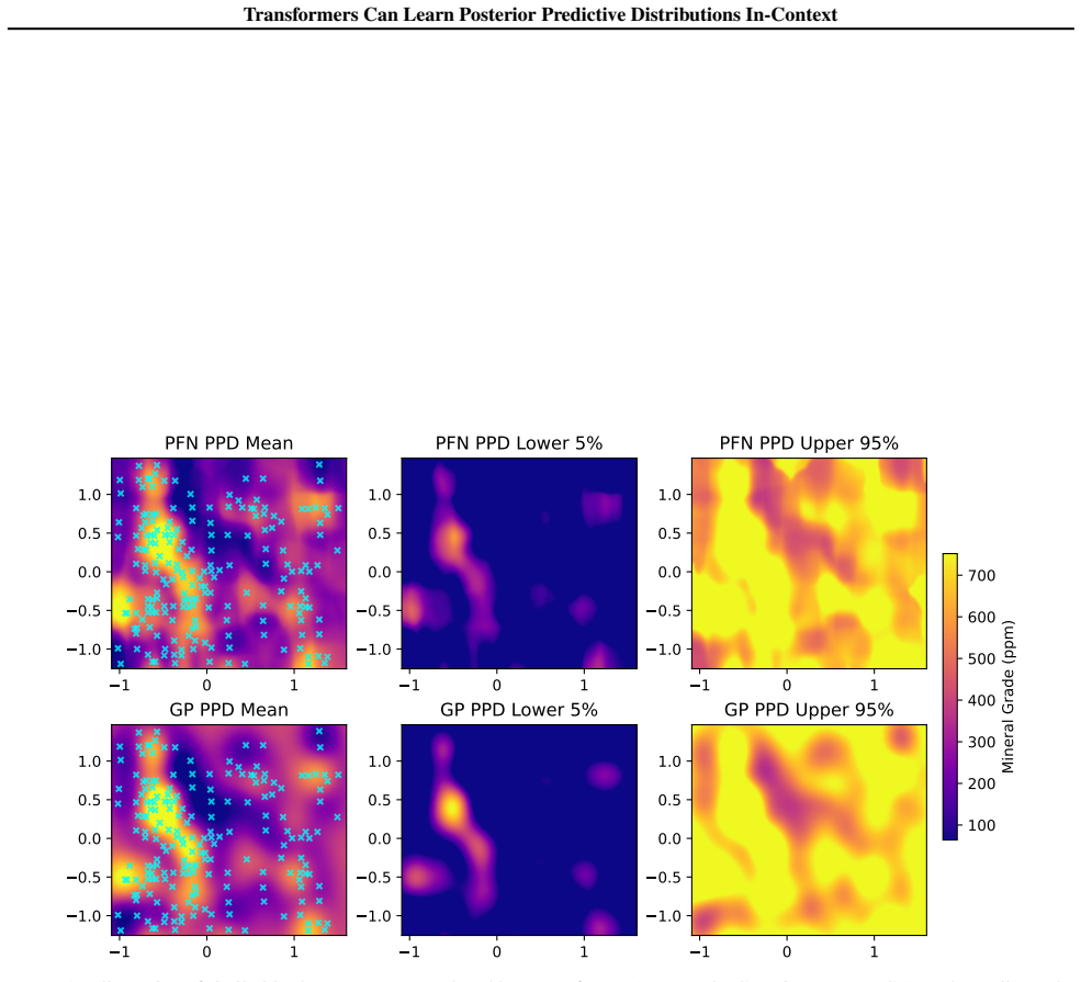
Note that this case study is intended as an illustrative validation of the proposed mechanism rather than as a comprehensive benchmark
and the Walker Lake dataset (Isaaks & Srivastava, 1989). Note that this case study is intended as an illustrative validation of the proposed mechanism rather than as a comprehensive benchmark. Sacramento.The dataset is from the R package caret version 7.0.1 (Kuhn, 2008), from which we selected data corresponding to the cities of Sacramento and Elk Grove. ...
1989
-
[12]
Following Rasmussen & Williams (2005, Chapter 5), we first fit an empirical-Bayes anisotropic RBF GP to the Sacramento data
This preprocessing is used consistently for empirical-Bayes fitting, PFN pretraining, and evaluation. Following Rasmussen & Williams (2005, Chapter 5), we first fit an empirical-Bayes anisotropic RBF GP to the Sacramento data. Specifically, we use the ARD kernel κ(x, x′) =α 2 exp −1 2 2X k=1 (xk −x ′ k)2 ℓ2 k ! , together with Gaussian observation noise. ...
2005
-
[13]
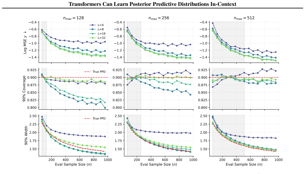
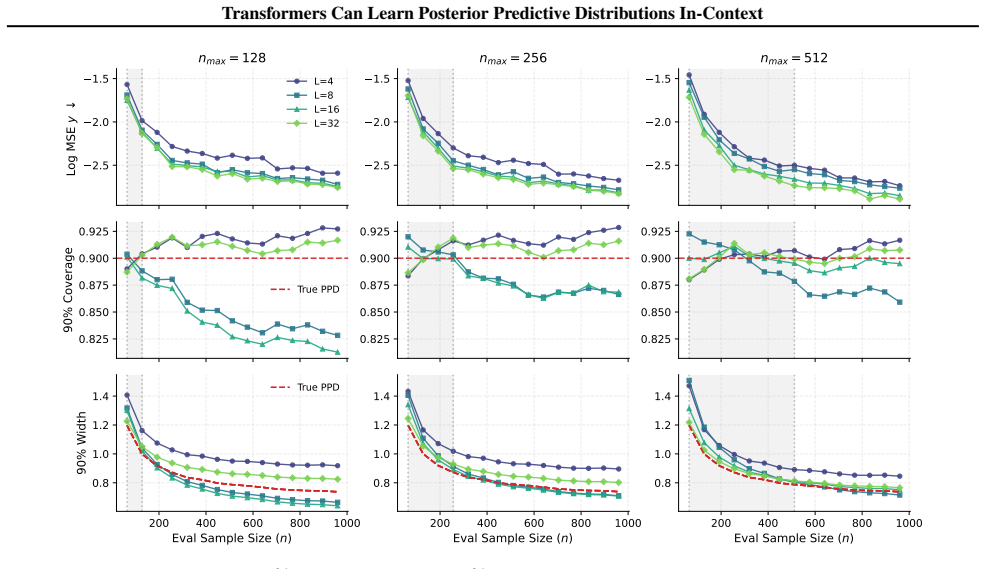
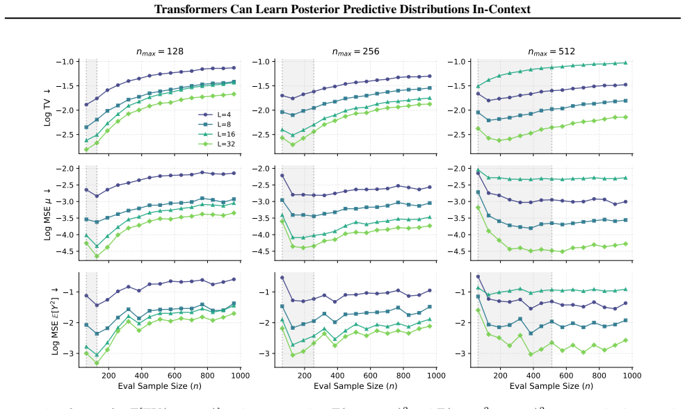
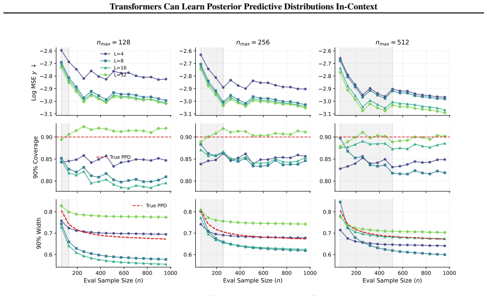
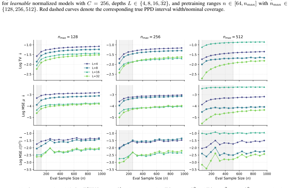
Consistent with Theorem 5.3, for fixed L and nmax, the error of the finite-iteration solver increases as the evaluation sample size grows. 29 Transformers Can Learn Posterior Predictive Distributions In-Context 3.1 3.0 2.9 2.8 2.7 2.6 Log MSE y nmax = 128 L=4 L=8 L=16 L=32 3.1 3.0 2.9 2.8 2.7 2.6 nmax = 256 3.1 3.0 2.9 2.8 2.7 2.6 nmax = 512 0.80 0.85 0.9...
1989
discussion (0)
Sign in with ORCID, Apple, or X to comment. Anyone can read and Pith papers without signing in.