REVIEW 3 major objections 6 minor 2 references
A dedicated neural network for the certainty equivalent lets deep learning solve recursive-utility dynamic programs, including occasionally binding constraints, via first-order and KKT residuals.
Reviewed by Pith at T0; open to challenge. T0 means a machine referee read the full paper against a public rubric. the ladder, T0–T4 →
T0 review · grok-4.5
2026-07-13 02:51 UTC pith:HOJYQAUK
load-bearing objection Solid methods paper: separate CE network into FOC/KKT residual learning for constrained recursive-utility DP; residual evidence is real but soft, VFI only on one low-dim case. the 3 major comments →
Deep Learning for Dynamic Programming with Recursive Utility Using First-order Conditions
The pith
A machine-rendered reading of the paper's core claim, the machinery that carries it, and where it could break.
Core claim
Representing the state-control certainty equivalent by a dedicated neural network, and feeding that approximation into model-specific first-order and KKT residual losses for the policy and multipliers, produces a practical deep-learning solver for discrete-time recursive-utility dynamic programming that handles general equality and inequality constraints, including occasionally binding ones, with small residual diagnostics and close agreement with VFI when available.
What carries the argument
The certainty-equivalent first-order learning (CEFOL) scheme: a certainty-equivalent network C(s,c) that amortizes the nonlinear transformation f⁻¹(E[f(V(s′))]), combined with residual losses built from stationarity (including Euler), Fischer–Burmeister complementarity, and equality constraints, trained with target networks and delayed policy updates.
Load-bearing premise
That small out-of-sample residual diagnostics under nonconvex neural training, plus optional agreement with grid VFI on low-dimensional cases, are enough to treat the learned networks as accurate solutions of the true recursive program.
What would settle it
On any of the reported models, recompute nested Monte Carlo Bellman and Euler/KKT residuals (or a high-resolution VFI benchmark) on an independent dense test set; if residuals remain large or systematically biased away from the training residual classes, or if policies diverge from VFI where VFI is reliable, the claim fails.
Editorial analysis
A structured set of objections, weighed in public.
Referee Report
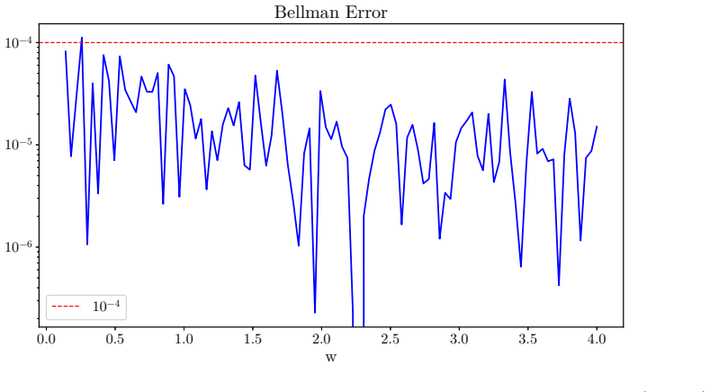
Summary. The paper proposes CEFOL, a deep learning algorithm for discrete-time infinite-horizon dynamic programs with recursive utility. The central device is a dedicated neural network for the state-control certainty-equivalent value C(s,c), which is then inserted into Bellman targets and into model-specific first-order/KKT residuals used to train policy and multiplier networks. Value, certainty-equivalent, and (when used) multiplier networks are trained on separate residual losses, with stabilizations including target value networks, delayed FOC updates, exploratory control perturbation, and an independent sample-mean product estimator for squared conditional stationarity residuals. The framework is written for general equality/inequality constraints and occasionally binding constraints via Fischer–Burmeister KKT terms. Numerical applications cover risk-sensitive and Epstein–Zin consumption-saving models, a small-noise robust-control problem (with VFI benchmarks), and an Epstein–Zin DSGE model with stochastic volatility. Reported out-of-sample Bellman and FOC/Euler residuals are typically of order 10^{-4}–10^{-3} over relevant state regions, with larger residuals mainly near binding constraints, and close agreement with VFI when available.
Significance. If the method works as claimed, it is a useful computational contribution for recursive-utility dynamic programming, where nonlinear certainty equivalents enter both the Bellman equation and optimality conditions and are hard to evaluate inside policy updates. The careful FOC/KKT derivation under recursive utility (§2.2), including the structural condition that can eliminate future value gradients, and the modular treatment of vector controls and occasionally binding constraints without penalty reformulations, are genuine strengths relative to expected-utility residual methods and to model-specific deep equilibrium systems. The paper also situates CEFOL relative to Maliar et al. (2021), Friedl et al. (2023), and the companion CEL algorithm, and shows that expected utility is nested. For a computational journal, residual diagnostics plus VFI agreement on a low-dimensional nonlinear case are a recognizable evaluation package; the main open issue is how tightly residual smallness pins down solution accuracy for the harder recursive models.
major comments (3)
- [§4 Numerical Results; §3.2–3.3] §3.2–3.3 and §4: The headline accuracy claim (Abstract; §4) rests on out-of-sample Bellman and FOC/Euler residuals of order 10^{-4}–10^{-3}, plus VFI agreement only in the small-noise robust-control model (§4.3). Those residual classes are essentially the same objectives minimized in training (certainty-equivalent, Bellman, stationarity, Fischer–Burmeister). Nested simulation improves the diagnostic estimator relative to the training product estimator, but still measures consistency of a learned fixed point rather than distance to the true value/policy. For the risk-sensitive, Epstein–Zin consumption-saving, and DSGE applications, the paper relies on internal CEFOL/CEFOL-td/CEFOL-vc alignment and residual size. Given the paper’s own acknowledgment of nonconvex training without global optimality guarantees (§1), the accuracy claim needs stronger independent grounding: multi-seed/hyperpara
- [§2.2; applications in §4.1–4.4] §2.2, Eqs. (18)–(27): The FOC simplification that eliminates ∂V(s_{t+1})/∂s_{t+1} depends on a structural condition that the transition factors through a scalar y_{t+1}. This is load-bearing for the practical residual forms used later. The applications in §4.1–4.4 implement specialized Euler/KKT residuals, but the manuscript does not systematically verify that (18) holds in each environment or state what is done when it fails (direct automatic differentiation of C and V, alternative envelope forms, etc.). Please state explicitly, for each numerical model, whether the structural condition is used, how F_{t+1,k} is obtained, and whether any residual involves future value gradients.
- [§3.1; §4; literature discussion of CEL/Friedl] §3.1 and §4: Three architectures are developed (four-, five-, and three-network), yet the numerical section appears to use only the four-network baseline. Without ablations, the five-network decomposition (Ve, D) and the compact three-network variant remain untested design options rather than demonstrated tools. Either report comparative residuals/stability/cost for the alternative architectures on at least one application, or narrow the main text to the architecture actually used and move the others to an appendix as optional variants. Relatedly, CEFOL is positioned as complementary to CEL (Peng and Guo, 2026) and distinct from Friedl et al. (2023), but §4 contains no head-to-head accuracy or cost comparison on a shared recursive-utility problem; such a comparison would substantially strengthen the methods contribution.
minor comments (6)
- [§4 figures and captions] Figures in §4 often evaluate along a one-dimensional slice (cash-on-hand or capital) with other states fixed at steady state. Please state this limitation more prominently when interpreting residual magnitudes, and consider reporting residual quantiles on simulated ergodic samples as a complement.
- [§3.4–3.5; §4] Hyperparameters (network widths/depths, learning rates, delay d, τ, residual weights λ_S/λ_FB, exploration ζ_k, N_z, etc.) are numerous but only partially documented in the main text. A compact table of training settings per application would aid reproducibility.
- [§4 opening; §4.1.3] In the risk-sensitive examples, absolute Bellman errors are used because V crosses zero; in other examples relative Bellman errors are used. A short note unifying the diagnostic definitions and normalizations (including the Euler residual (106)–(108)) would help cross-model comparison.
- [§2–§3] Notation occasionally shifts between C(s,c), C(s,c;θ_C), and script C; keep a single convention for the true certainty equivalent versus the network approximator.
- [title page] The manuscript date line reads “July 13, 2026”; confirm versioning/arXiv metadata consistency before journal submission.
- [§4 figures] Some figure panels mark horizontal thresholds (e.g., 10^{-4}, 10^{-3}) without stating whether these are formal tolerances or visual guides; clarify in captions.
Circularity Check
Residual training objectives reappear as out-of-sample diagnostics (standard for residual methods); VFI supplies limited external grounding and companion CEL is complementary, not load-bearing.
specific steps
-
other
[Abstract; §3.2–3.3 (losses); §4 (diagnostics)]
"By using first-order and KKT residuals to learn the policy... out-of-sample Bellman diagnostics and model-specific optimality residuals, including Euler or first-order residuals where applicable, are generally of order 1.0e-4 to 1.0e-3"
Training explicitly minimizes the certainty-equivalent, Bellman and FOC/KKT residual losses; the headline accuracy claim is that the same residual classes are small out-of-sample. For residual methods this is expected rather than a forced identity, but the diagnostic is not fully independent of the training objective (except where VFI is available).
full rationale
The paper derives model-specific FOC/KKT residuals from the recursive Bellman equation (§2.2), then trains networks by minimizing certainty-equivalent, Bellman, stationarity and Fischer–Burmeister losses (§3.2–3.3). Evaluation reports the same residual classes on independent test states plus nested simulation (§4), together with internal consistency (CEFOL vs CEFOL-td vs CEFOL-vc) and VFI agreement only for the small-noise robust-control model (§4.3). This is the ordinary residual-method loop, not a self-definitional identity or a fitted parameter renamed as prediction: out-of-sample states and a different Monte-Carlo estimator keep the diagnostics from being literally identical to the training loss. The companion CEL citation (Peng & Guo 2026) is explicitly complementary (Bellman maximization versus FOC residuals) and is not used to force uniqueness or forbid alternatives. No uniqueness theorem is imported from the authors, no ansatz is smuggled via self-citation, and the FOC derivation itself is self-contained. Score 2 reflects only the mild, expected self-reference of residual diagnostics; the central algorithmic claim retains independent content via the separate certainty-equivalent network and the VFI benchmark where available.
Axiom & Free-Parameter Ledger
free parameters (6)
- Neural network architectures and widths/depths for V, c, m, C (and optional Ve, D)
- Learning rates α_V, α_c, α_m, α_C (and α_e, α_D) and optimizer settings
- FOC update delay d and target soft-update rate τ
- Residual weights λ_S, λ_FB, λ_EQ and component normalizers v_S, v_FB, v_EQ
- Exploration scale ζ_k and path-simulation design (N, N_z, mini-batching)
- Model preference/technology calibrations (e.g., σ, β, γ, ρ, ψ, DSGE parameters)
axioms (6)
- domain assumption Recursive utility admits a Bellman representation V(s)=max_c w(s,c,C(s,c)) with C=f^{-1}(E[f(V(s'))|s,c]).
- domain assumption Relevant functions are differentiable and derivatives may pass through conditional expectations when forming FOCs.
- domain assumption Optional structural condition: next-state map factors through a scalar y(s,c) so future value gradients can be eliminated via envelope and next-period stationarity.
- standard math KKT conditions characterize the constrained optimum (stationarity, primal feasibility, dual feasibility, complementarity).
- standard math Conditionally independent residual product estimates the squared conditional mean residual (all-in-one / independent sample-mean estimator).
- ad hoc to paper Neural-network residual minimization yields a practically accurate solution despite nonconvex training.
invented entities (2)
-
CEFOL multi-network architecture with dedicated state-control certainty-equivalent network
no independent evidence
-
Five-network CE decomposition into conditional expectation Ve and nonlinear difference D
no independent evidence
read the original abstract
This paper proposes the certainty-equivalent first-order learning (CEFOL) algorithm, a deep learning algorithm for solving discrete-time dynamic programming problems with recursive utility. Dynamic programming with recursive utility is challenging because nonlinear certainty equivalent appears in the Bellman equation and the first-order optimality conditions but is difficult to evaluate. By introducing a separate neural network to represent the certainty equivalent, CEFOL enables the exploitation of the Bellman and model-specific first-order optimality conditions. In addition to certainty equivalent, CEFOL also uses neural networks to learn the value functions, policy functions, and Lagrange multipliers by using model-specific first-order conditions to construct residuals for minimization. By using first-order and KKT residuals to learn the policy, CEFOL directly accommodates general equality and inequality constraints on the controls, including occasionally binding constraints, without requiring penalty functions or problem-specific reformulations. We apply the algorithm to risk-sensitive and Epstein--Zin consumption-saving problems, a small-noise robust-control problem, and a DSGE model with recursive preferences and stochastic volatility. Across these applications, out-of-sample Bellman diagnostics and model-specific optimality residuals, including Euler or first-order residuals where applicable, are generally of order 1.0e-4 to 1.0e-3 over the relevant state regions, with larger values mainly near binding constraints, and the learned value and policy functions closely match VFI benchmarks when available. The CEFOL algorithm also works for dynamic programming problems with expected utility, as expected utility is a special case of recursive utility.
Figures




Reference graph
Works this paper leans on
-
[1]
Aboussalah, A. M., Xu, Z. and Lee, C.-G. (2022). What is the value of the cross-sectional approach to deep reinforcement learning?,Quantitative Finance22(6): 1091–1111. Andreasen, M. M. (2012). On the effects of rare disasters and uncertainty shocks for risk premia in non-linear dsge models,Review of Economic Dynamics15(3): 295–316. Azinovic, M., Gaegauf,...
Pith/arXiv arXiv 2022
-
[2]
Dumas, B., Uppal, R. and Wang, T. (1998). Efficient intertemporal allocations with recursive utility. E, W., Han, J. and Jentzen, A. (2017). Deep learning-based numerical methods for high- dimensional parabolic partial differential equations and backward stochastic differential equations,Communications in Mathematics and Statistics5(4): 349–380. Epstein, ...
Pith/arXiv arXiv 1998
discussion (0)
Sign in with ORCID, Apple, or X to comment. Anyone can read and Pith papers without signing in.